Big Data

Big data primarily refers to data sets that are too large or complex to be dealt with by traditional data-processing application software. Big data analysis challenges include capturing data, data storage, data analysis, search, sharing, transfer, visualization, querying, updating, information privacy, and data source.

Big data can be described by following characteristics:

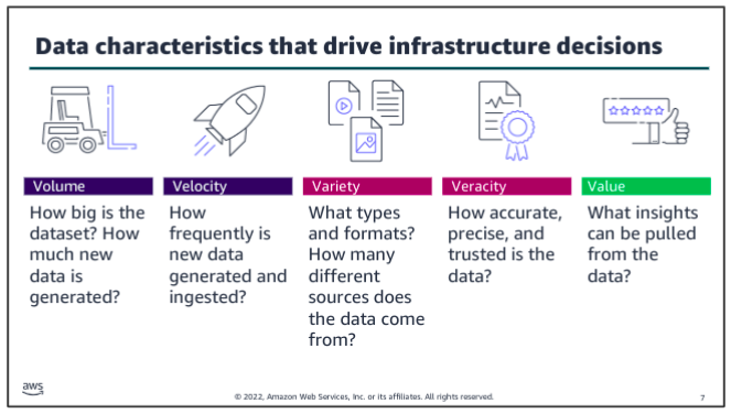
• Volume: The quantity of generated and stored data. The size of the data determines the value and potential insight, and whether it can be considered big data or not. The size of big data is usually larger than terabytes and petabytes.

• Variety: The type and nature of the data. Earlier technologies like RDBMSs were capable to handle structured data efficiently and effectively. However, the change in type and nature from structured to semi-structured or unstructured challenged the existing tools and technologies. Big data technologies evolved with the prime intention to capture, store, and process the semi-structured and unstructured (variety) data generated with high speed (velocity), and huge in size (volume).

• Velocity: The speed at which the data is generated and processed to meet the demands and challenges that lie in the path of growth and development. Big data is often available in real-time. Compared to small data, big data is produced more continually. Two kinds of velocity related to big data are the frequency of generation and the frequency of handling, recording, and publishing.

• Veracity: The truthfulness or reliability of the data, which refers to the data quality and the data value. Big data must not only be large in size, but also must be reliable in order to achieve value in the analysis of it. The data quality of captured data can vary greatly, affecting an accurate analysis.

• Value: The worth in information that can be achieved by the processing and analysis of large datasets. Value also can be measured by an assessment of the other qualities of big data.  Value may also represent the profitability of information that is retrieved from the analysis of big data.

Other possibles:

• Visualization, Exhaustive, Fine-grained, Scalability, Extensional

Take one at a time:

• Consider volume and velocity together because you will make infrastructure decisions about how to collect, store, and process data based on the combination of how much data you need to ingest and how quickly you will ingest it.
• Variety and veracity both relate to the data itself - what type of data is it and what’s the quality of it. Data engineers and data scientists will transform and organize the data based on its variety and veracity to make it useful for analysis.
• Value is about ensuring that you are getting the most out of the data that you have collected. Value is also about ensuring that there is business value in the outputs from all that collecting, storing, and processing.

vs business intelligence:

Business Intelligence uses applied mathematics and descriptive statistics with data with high information density to measure things, detect trends, etc. Big data uses mathematical analysis, optimization, inductive statistics, and concepts from nonlinear system identification to infer laws (regressions, nonlinear relationships, and casual effects) from large sets of data with low information density to reveal relationships and dependencies, or to perform predictions of outcomes and behaviors.

Analytics

Current usage of the term big data tends to refer to the use of predictive analytics, user behavior analytics, or certain other advanced data analytics methods that extract value from big data, and seldom to a particular size of data set. Analysis of data sets can find new correlations to spot business trends, prevent diseases, combat crime and so on.

Data analytics:

• is the systematic analysis of large datasets (big data) to find patterns and trends to produce actionable insights
• uses programming logic to answer questions from data
• is good for structured data with a limited number of variables

AI/ML:

• is a set of fundamental models that are used to make predictions from data at a scale that is difficult or impossible for humans
• uses examples from large amounts of data to learn about the data and answer questions
• is good for unstructured data and where the variables are complex

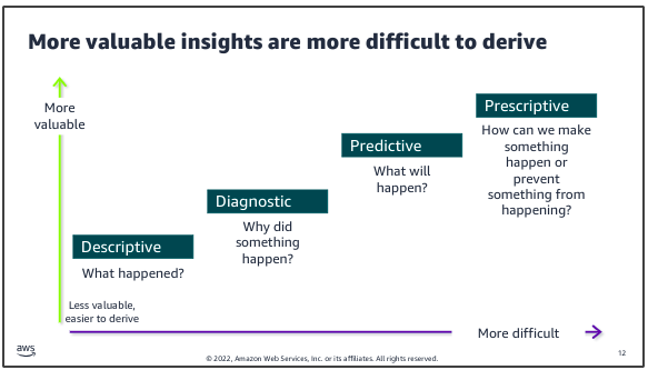
Descriptive: summarizes historical data to understand what has happened in the past.

• Techniques: data aggregation, data mining, reports, dashboards
• Examples: sales reports showing revenue numbers, engagement metrics, customer survey scores

Diagnostic: focuses on understanding why certain events or outcomes occurred.

• Techniques: hypothesis testing, correlation, regression analysis
• Examples: drivers behind market spikes, root cause of IT issues

Predictive: aims to forecast future events or trends based on historical data.

• Techniques: predictive modeling, machine learning, forecasting models
• Examples: credit risk models, future market demands, supply chain planning

Prescriptive: seeks to determine the best course of action or decision to take.

• Techniques: simulation methods, recommendation engines, optimization and operations
• Examples: rules engines triggering marketing campaign, constraint based optimization

Applications

Big data has increased the demand of information management specialists so much that software firms have spent more than $15billionspecializingindatamanagementandanalytics.In2010,thisindustrywasworthmorethan$100 billion and was growing at almost 10 percent a year, about twice as fast as the software business as a whole.

Finance:

• investing decisions and trading, price data, limit order books, economic data and more
• portfolio management, large array of financial instruments
• risk management

Healthcare:

• personalized medicine and prescriptive analytics
• clinical risk intervention
• predictive analytics
• waste and care variability reduction
• automated external and internal reporting of patient data

Education:

• master bootcamps

Media:

• data capture and data journalism

Internet of Things:

• sensor data in manufacturing and transportation contexts

Marketing:

• behavior pattern spotting
• real-time market responsiveness
• market driven ambidexterity

Science:

• LHC sensors
• satellite feeds
• genome data
• computational fluid dynamics

A particular business case:

Walmart handles more than 1 million customer transactions every hour, which are imported into databases estimated to contain more than 2.5 petabytes of data. Walmart was the world’s largest retailer in terms of revenue. It makes $36 million dollars from across 4300 retail stores in US, daily and employs close to 2 million people. In 2012 Walmart made a move from experiental 10 node Hadoop cluster to a 250 node Hadoop cluster. Since then, Walmart has been speeding along big data analysis to provide best-in-class e-commerce technologies with a motive to deliver pre-eminent customer experience.

Walmart acquired a small startup Inkiru based in Palo Alto, California to boost its big data capabilites. Inkiru Inc. helps in targeted marketing, merchandising and fraud prevention. Inkiru’s predictive technology platform pulls data from diverse sources and helps Walmart improve personalization through data analytics. The predictive analytics platforrm of Inkiru incorporates machine learning technologies to automatically enhance the accuracy of algorithms and can integrate with diverse external and internal data sources.

Walmart has transformed decision making in the business world resulting in repeated sales. Walmart observed a significant 10% to 15% increase in online sales for $1 billion in incremental revenue. Big data analysts were able to identify the value of the changes Walmart made by analysing the sales before and after big data analytics were leveraged to change the retail giant’s e-commerce strategy.

Distributed concepts for big data? (study Distributed Systems at this point then only move on)

Google Case Study

From a distributed systems perspective, Google provides a fascinating case study with extremely demanding requirements, particularly in terms of

• scalability,
• reliability,
• performance and
• openness

The Google search engine: The role of the Google search engine is, as for any web search engine, to take a query and return an ordered list of the most relevant results that match that query by searching the content of the Web. The challenges stem from the size of the Web and its rate of change, as well as the requirement to provide the most relevant results from the perspective of its users.

Crawling: The task of the crawler is to locate and retrieve the contents of the Web and pass the contents onto the indexing subsystem. This is performed by a software service called Googlebot, which recursively reads a given web page, harvesting all the links from that web page and then scheduling further crawling operations for the harvested links (a technique known as deep searching that is highly effective in reaching practically all pages in the Web). In the past, because of the size of the Web, crawling was generally performed once every few weeks. However, for certain web pages this was insufficient. For example, it is important for search engines to be able to report accurately on breaking news or changing share prices. Googlebot therefore took note of the change history of web pages and revisited frequently changing pages with a period roughly proportional to how often the pages change. With the introduction of Caffeine in 2010, Google has moved from a batch approach to a more continuous process of crawling intended to offer more freshness in terms of search results.

Indexing: The role of indexing is to produce an index for the contents of the Web that is similar to an index at the back of a book, but on much larger scale. More precisely, indexing produces what is known as an inverted index mapping words appearing in web pages and other textual web resources (including documents in .pdf, .doc and other formats) onto the positions where they occur in documents, including the precise position in the document and other relevant information such as the font size and capitalization (which is used to determine importance, as will be seen below). The index is also sorted to support efficient queries for words against locations.

Example: This inverted index will allow us to discover web pages that include the search terms ‘distributed’, ‘systems’ and ‘book’ and, by careful analysis, we will be able to discover pages that include all of these terms. The search engine will be able to identify that the three terms can all be found in amazon.com, cdk5.net and indeed many other web sites. Using the index, it is therefore possible to narrow down the set of candidate web pages from billions to perhaps tens of thousands, depending on the level of discrimination in the keywords chosen.

Ranking: The problem with indexing on its own is that it provides no information about the relative importance of the web pages containing a particular set of keywords – yet this is crucial in determining the potential relevance of a given page. All modern search engines therefore place significant emphasis on a system of ranking whereby a higher rank is an indication of the importance of a page and it is used to ensure that important pages are returned nearer to the top of the list of results than lower-ranked pages. PageRank is inspired by the system of ranking academic papers based on citation analysis. In the academic world, a paper is viewed as important if it has a lot of citations by other academics in the field. Similarly, in PageRank, a page will be viewed as important if it is linked to by a large number of other pages (using the link data mentioned above). PageRank also goes beyond simple ‘citation’ analysis by looking at the importance of the sites that contain links to a given page. For example, a link from bbc.co.uk will be viewed as more important than a link from Gordon Blair’s personal web page.

Anatomy of a search engine: The founders of Google, Sergey Brin and Larry Page, wrote a seminal paper on the anatomy of Google search engine in 1998, providing interesting insights into how their search engine was implemented. The overall architecture described in this paper is:

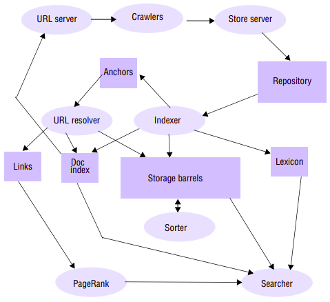
(explanations)

Google as a cloud provider:

Google services:

Design Philosophy

The key philosophy of Google in terms of physical infrastructure is to use very large number of commodity PCs to produce a cost-effective environment for distributed storage and computation. Purchasing decisions are based on obtaining the best performance per dollar rather than absolute performance with a typical spend PC unit of $1,000. A given PC will typically have 2 terabytes of disk storage and around 16 gigabytes of DRAM and run a cut down version of Linux kernel. This philosophy of building systems from commodity PCs reflects the early days of the original research project, when Sergey Brin and Larry Page built the first Google search engine from spare hardware scavenged from around the lab at Stanford University.

In electing to go down the route of commodity PCs, Google has recognized that parts of its infrastructure will fail and hence, has designed the infrastructure using a range of strategies to tolerate such failures. Hennessy and Patterson report the following failure characteristics for Google:

• By far the most common source of failure is due to software, with about 20 machines needing to be rebooted per day due to software failures. (Interestingly, the rebooting process is entirely manual.)
• Hardware failures represent about 1/10 of the failures due to software with around 2–3% of PCs failing per annum due to hardware faults. Of these, 95% are due to faults in disks or DRAM.

This vindicates the decision to procure commodity PCs; given that the vast majority of failures are due to software, it is not worthwhile to invest in more expensive, more reliable hardware.

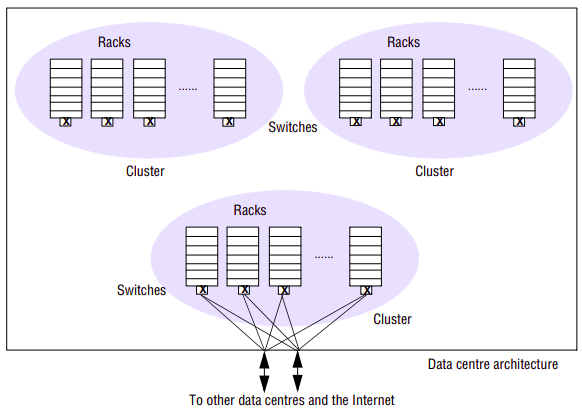
The physical architecture is constructed as follows:

Commodity PCs are organized in racks with between 40 and 80 PCs in a given rack. The racks are double-sided with half the PCs on each side. Each rack has an Ethernet switch that provides connectivity across the rack and also to the external world. This switch is modular, organized as a number of blades with each blade supporting either 8 100-Mbps network interfaces or a single 1-Gbps interface. For 40 PCs, five blades each containing eight network interfaces are sufficient to ensure connectivity within the rack. Two further blades, each supporting a 1-Gbps network interface, are used for connection to the outside world.

Racks are organized into clusters, which are a key unit of management, determining for example the placement and replication of services. A cluster typically consists of 30 or more racks and two high-bandwidth switches providing connectivity to the outside world (the Internet and other Google centres). Each rack is connected to both switches for redundancy; in addition, for further redundancy, each switch has redundant links to the outside world.

Clusters are housed in Google data centres that are spread around the world. In 2000, Google relied on key data centres in Silicon Valley (two centres) and in Virginia. At the time of writing, the number of data centres has grown significantly and there are now centres in many geographical locations across the US and in Dublin (Ireland), Saint-Ghislain (Belgium), Zurich (Switzerland), Tokyo (Japan) and Beijing (China).

Let us consider the storage capacity available to Google. If each PC offers 2 terabytes of storage, then a rack of 80 PCs will provide 160 terabytes, with a cluster of 30 racks offering 4.8 petabytes. It is not known exactly how many machines Google has in total as the company maintains strict secrecy over this aspect of its business, but we can assume Google has on the order of 200 clusters, offering total storage capacity of 960 petabytes or just under 1 exabyte of storage.

System Architecture

Requirements for system?

Scalability:

The first and most obvious requirement for the underlying Google infrastructure is to master scalability and, in particular, to have approaches that scale to what is an Ultra-Large Scale (ULS) distributed system. For the search engine, Google views the scalability problem in terms of three dimensions:

• being able to deal with more data (for example, as the amount of information in the Web grows through initiatives such as the digitizing of libraries),
• being able to deal with more queries (as the number of people using Google in their homes and workplaces grows) and
• seeking better results (particularly important as this is a key determining factor in uptake of a web search engine).

Reliability:

Google has stringent reliability requirements, especially with regard to availability of services. This is particularly important for the search functionality, where there is a need to provide 24/7 availability (noting, however that it is intrinsically easy to mask failures in search as the user has no way of knowing if all search results are returned).

Performance:

The overall performance of the system is critical for Google, especially in achieving low latency of user interactions. The better the performance, the more likely it is that a user will return with more queries that, in turn, increase their exposure to ads hence potentially increasing revenue.

Openenss:

The above requirements are in many ways the obvious ones for Google to support its core services and applications. There is also a strong requirement for openness, particularly to support further development in the range of web applications on offer. It is well known that Google as an organization encourages and nurtures innovation, and this is most evident in the development of new web applications.

Google has responded to these needs by developing the overall system architecture:

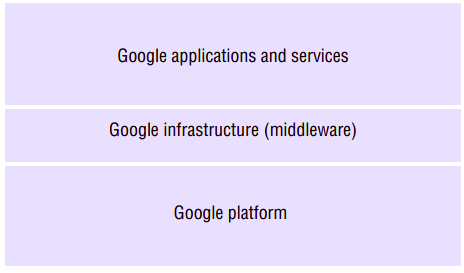
Google infrastructure:

(more explanations)

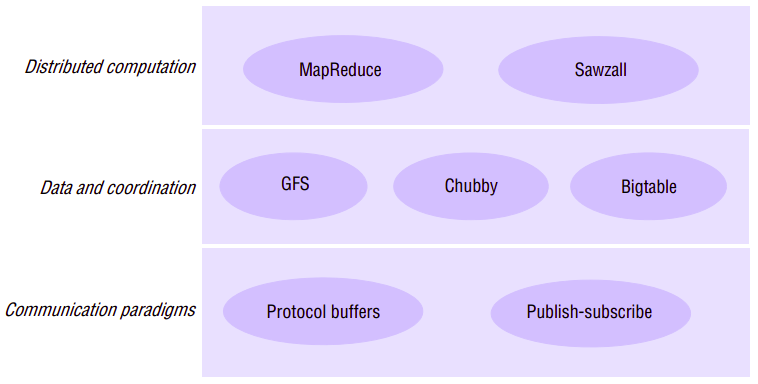
Data Storage and Coordination Services

The three services that together provide data and coordination services to higher-level applications and services: the Google File System, Chubby and Bigtable. These are complementary services in the Google infrastructure:

• The GFS is a distributed file system offering a similar service to NFS and AFS. It offers access to unstructured data in the form of files, but optimized tot he styles of data and data access required by Google (very large files, for example).
• Chubby is a multi-faceted service supporting, for example, coarse-grained distributed locking for coordination in the distributed environment and the storage of very small quantities of data, complementing the large-scale storage offered by the GFS.
• Bigtable offers access to more structured data in the form of tables that can be indexed in various ways including by row or column. Bigtable is therefore a style of distributed database, but unlike many databases it does not support full relational operators (these are viewed by Google as unnecessarily complex and unscalable ).

These three services are also interdependent. For example, Bigtable uses the Google File System for storage and Chubby for coordination.

The Google File System

The NFS and AFS are general-purpose distributed file systems offering file and directory abstractions to a wide variety of applications in and across organizations. The GFS is also a distributed file system; it offers similar abstractions but is specialized for the very particular requirement that Google has in terms of storage and access to very large quantities of data. These requirements led to very different design decisions from those made in NFS and AFS.

The overall goal of GFS is to meet the demanding and rapidly growing needs of Google’s search engine and the range of other web applications offered by the company. From an understanding of this particular domain of operation, Google identified the following requirements for GFS:

• The first requirement is that GFS must run reliably on the physical architecture - that is a very large system built from commodity hardware. The designers of GFS started with the assumption that components will fail (not just hardware but also software components) and that the design must be sufficiently tolerant of such failures to enable application-level services to continue their operation in the face of any likely combination of failure conditions.
• GFS is optimized for the patterns of usage within Google, both in terms of the types of files stored and the patterns of access to those files. The number of files stored in GFS is not huge in comparison with other systems, but the files tend to be massive. For example, Ghemawat report the need for perhaps one million files averaging 100 megabytes in size, but with some files in the gigabyte range. The patterns of access are also atypical of file systems in general.
• Accesses are dominated by sequential reads through large files and sequential writes that append data to files, and GFS is very much tailored towards this style of access. Small, random reads and writes do occur (the latter very rarely) and are supported, but the system is not optimized for such cases. These file patterns are influenced, for example, by the storage of many web pages sequentially in single files that are scanned by a variety of data analysis programs.
• The level of concurrent access is also high in Google, with large numbers of concurrent appends being particularly prevalent, often accompanied by concurrent reads. Atomicity with minimal synchronization overhead is essential. The file may be read later, or a consumer may be reading through the file simultaneously.
• GFS must meet all the requirements for the Google infrastructure as a whole; that is, it must scale (particularly in terms of volume of data and number of clients), it must be reliable in spite of the assumption about failures noted above, it must perform well and it must be open in that it should support the development of new web applications. In terms of performance and given the types of data file stored, the system is optimized for high and sustained throughput in reading data, and this is prioritized over latency. This is not to say that latency is unimportant, rather, that this particular component (GFS) needs to be optimized for high-performance reading and appending of large volumes of data for the correct operation of the system as a whole.

These requirements are markedly different from those for NFS and AFS (for example), which must store large numbers of often small files and where random reads and writes are commonplace.

Interface:

GFS provides a conventional file system interface offering a hierarchical namespace with individual files identified by pathnames. Although the file system does not provide full POSIX compatibility, many of the operations will be familiar to users of such file systems. It supports the usual operations to create, delete, open, close, read, and write files. Morever, GFS has snapshot and record append operations. Snapshot creates a copy of a file or a directory tree at low cost. Record append allows multiple clients to append data to the same file concurrently while guaranteeing the atomicity of each individual client’s append. It is useful for implementing multi-way merge results and producerconsumer queues that many clients can simultaneously append to without additional locking.

Chunk size:

The most influential design choice in GFS is the storage of files in fixed-size chunks, where each chunk is 64 megabytes in size. This is quite large compared to other file system designs. At one level this simply reflects the size of the files stored in GFS. At another level, this decision is crucial to providing highly efficient sequential reads and appends of large amounts of data.

Given this design choice, the job of GFS is to provide a mapping from files to chunks and then to support standard operations on files, mapping down to operations on individual chunks.

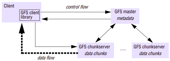
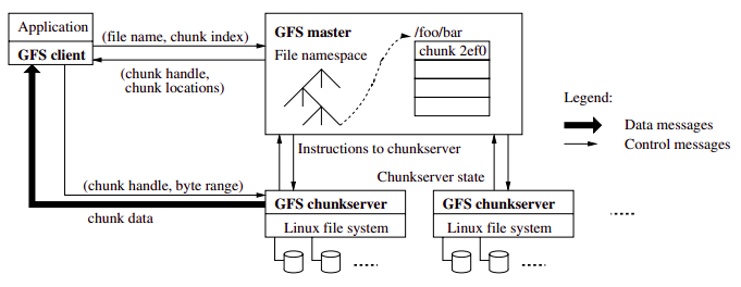
An instance of a GFS file system as it maps onto a given physical cluster. GFS cluster has a single master and multiple chunkservers (typically on the order of hundreds), which together provide a file service to large numbers of clients concurrently accessing the data. The role of the master is to manage metadata about the file system defining the namespace for files, access control information and the mapping of each particular file to the associated set of chunks.

Note that one further repercussion of the large chunk size is that GFS maintains proportionally less metadata (if a chunk size of 64 kilobytes was adopted, for example, the volume of metadata would increase by a factor of 1,000). This in turn implies that GFS masters can generally maintain all their metadata in main memory, thus significantly decreasing the latency for control operations.

In addition, all chunks are replicated (by default on three independent chunkservers, but the level of replication can be specified by the programmer). The location of the replicas is maintained in the master. Replication is important in GFS to provide the necessary reliability in the event of (expected) hardware and software failures. This is in contrast to NFS and AFS, which do not provide replication with updates.

Single master bottleneck:

The master stores three major types of metadata:

• the file and chunk namespaces
• the mapping from files to chunks
• the locations of each chunk’s replicas

The key metadata is stored persistently in an operation log that supports recovery in the event of crashes (again enhancing reliability). In particular, all the information mentioned above is logged apart from the location of replicas (the latter is recovered by polling chunkservers and asking them what replicas they currently store). The master does not keep a persistent record of which chunkservers have a replica of given chunk. It simply polls chunkservers fro that information at startup. The master can keep itself up-to-date thereafter because it controls all chunkplacement and monitors chunkserver status with regular HeartBeat messages.

Although the master is centralized, and hence a single point of failure, the operations log is replicated on several remote machines, so the master can be readily restored on failure. The master recovers its file system state by replaying the operation log. To minimize startup time, the log file is kept small. The master checkpoints its state whenever the log grows beyond a certain size so that it can recover by loading the latest checkpoint from local disk and replaying only the liimtied number of log records after that. The benefit of having such a single, centralized master is that it has a global view of the file system and hence it can make optimum management decisions, for example related to chunk placement. This scheme is also simpler to implement, allowing Google to develop GFS in a relatively short period of time.

Caching:

Caching often plays a crucial role in the performance and scalability of a file system. Interestingly, GFS does not make heavy use of caching. As mentioned above, information about the locations of chunks is cached at clients when first accessed, to minimize interactions with the master. Apart from that, no other client caching is used. In particular, GFS clients do not cache file data. Given the fact that most accesses involve sequential streaming, for example reading through web content to produce the required inverted index, such caches would contribute little to the performance of the system. Furthermore, by limiting caching at clients, GFS also avoids the need for cache coherency protocols.

GFS also does not provide any particular strategy for server-side caching (that is, on chunkservers) rather relying on the buffer cache in Linux to maintain frequently accessed data in memory.

Logging:

GFS is a key example of the use of logging in Google to support debugging and performance analysis. In particular, GFS servers all maintain extensive diagnostic logs that store significant server events and all RPC requests and replies. These logs are monitored continually and used in the event of system problems to identify the underlying causes.

Reads in GFS through RPC:

When clients need to access data starting from a particular byte offset within a file, the GFS client library will first translate this to a file name and chunk index pair (easily computed given the fixed size of chunks). This is then sent to the master in the form of an RPC request (using protocol buffers). The master replies with the appropriate chunk identifier and location of the replicas, and this information is cached in the client and used subsequently to access the data by direct RPC invocation to one of the replicated chunkservers. In this way, the master is involved at the start and is then completely out of the loop, implementing a separation of control and data flows – a separation that is crucial to maintaining high performance of file accesses. Combined with the large chunk size, this implies that, once a chunk has been identified and located, the 64 megabytes can then be read as fast as the file server and network will allow without any other interactions with the master until another chunk needs to be accessed. Hence interactions with the master are minimized and throughput optimized. The same argument applies to sequential appends.

Writes (or general mutations) in GFS (and managing consistency):

Given that chunks are replicated in GFS, it is important to maintain the consistency of replicas in the face of operations that alter the data – that is, the write and record append operations. GFS provides an approach for consistency management that:

• maintains the previously mentioned separation between control and data and hence allows high-performance updates to data with minimal involvement of masters;
• provides a relaxed form of consistency recognizing, for example, the particular semantics offered by record append.

The approach proceeds as follows:

When a mutation (i.e., a write, append or delete operation) is requested for a chunk, the master grants a chunk lease to one of the replicas, which is then designated as the primary. This primary is responsible for providing a serial order for all the currently pending concurrent mutations to that chunk. A global ordering is thus provided by the ordering of the chunk leases combined with the order determined by that primary. In particular, the lease permits the primary to make mutations on its local copies and to control the order of the mutations at the secondary copies; another primary will then be granted the lease, and so on.

GFS adopts a passive replication architecture with an important twist. In passive replication, updates are sent to the primary and the primary is then responsible for sending out subsequent updates to the backup servers and ensuring they are coordinated. In GFS, the client sends data to all the replicas but the request goes to the primary, which is then responsible for scheduling the actual mutations (the separation between data flow and control flow mentioned above). This allows the transmission of large quantities of data to be optimized independently of the control flow.

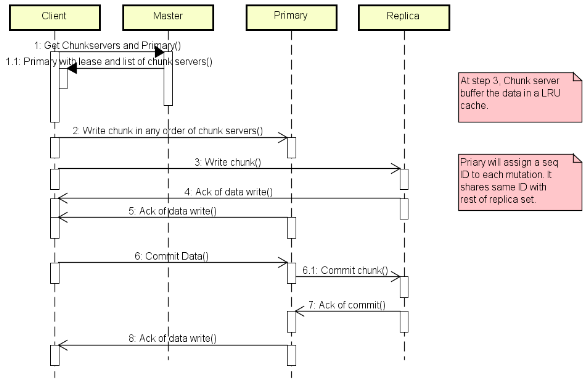
Stepwise:

• The client asks the master which chunkserver holds the current lease for the chunkand the locations of the other replicas. If no one has a lease, the master grants one to a replica it chooses.
• The master replies with the identity of the primary and the locations of the other (secondary) replicas. The client caches this data for future mutations. It needs to contact the master again only when the primary becomes unreachable or replies that it no longer holds a lease.
• The client pushes the data to all the replicas. A client can do so in any order. Each chunkserver will store the data in an internal LRU buffer cache until the data is used or aged out. By decoupling the data flow from the control flow, we can improve performance by scheduling the expensive data flow based on the networktopology regardless of which chunkserver is the primary.
• Once all the replicas have acknowledged receiving the data, the client sends a write request to the primary. The request identifies the data pushed earlier to all of the replicas. The primary assigns consecutive serial numbers to all the mutations it receives, possibly from multiple clients, which provides the necessary serialization. It applies the mutation to its own local state in serial number order.
• The primary forwards the write request to all secondary replicas. Each secondary replica applies mutations in the same serial number order assigned by the primary.
• The secondaries all reply to the primary indicating that they have completed the operation.
• The primary replies to the client. Any errors encountered at any of the replicas are reported to the client. In case of errors, the write may have succeeded at the primary and an arbitrary subset of the secondary replicas. (If it had failed at the primary, it would not have been assigned a serial number and forwarded.) The client request is considered to have failed, and the modified region is left in an inconsistent state. Our client code handles such errors by retrying the failed mutation. It will make a few attempts before failing back to a retry from the beginning of the write.

How data flows?

We decouple the flow of data from the flow of control to use the network efficiently. While control flows from the client to the primary and then to all secondaries, data is pushed linearly along a carefully picked chain of chunkservers in a pipelined fashion. Our goals are to fully utilize each machine’s network bandwidth, avoid network bottlenecks and high-latency links, and minimize the latency to push through all the data. To fully utilize each machine’s network bandwidth, the data is pushed linearly along a chain of chunkservers rather than distributed in some other topology (e.g., tree). Thus, each machine’s full outbound bandwidth is used to transfer the data as fast as possible rather than divided among multiple recipients.

To avoid network bottlenecks and high-latency links (e.g., inter-switch links are often both) as much as possible, each machine forwards the data to the “closest” machine in the networktopology that has not received it. Suppose the client is pushing data to chunkservers S1 through S4. It sends the data to the closest chunkserver, say S1. S1 forwards it to the closest chunkserver S2 through S4 closest to S1, say S2. Similarly, S2 forwards it to S3 or S4, whichever is closer to S2, and so on. Our networktopology is simple enough that “distances” can be accurately estimated from IP addresses.

Finally, we minimize latency by pipelining the data transfer over TCP connections. Once a chunkserver receives some data, it starts forwarding immediately. Pipelining is especially helpful to us because we use a switched networkwith full-duplex links. Sending the data immediately does not reduce the receive rate.

Consistency:

File namespace mutations (e.g., file creation) are atomic. They are handled exclusively by the master: namespace locking guarantees atomicity and correctness. The state of a file region after a data mutation depends on the type of mutation, whether it succeeds or fails, and whether there are concurrent mutations. A file region is consistent if all clients will always see the same data, regardless of which replicas they read from. A region is defined after a file data mutation if it is consistent and clients will see what the mutation writes in its entirety. When a mutation succeeds without interference from concurrent writers, the affected region is defined (and by implication consistent): all clients will always see what the mutation has written. Concurrent successful mutations leave the region undefined but consistent: all clients see the same data, but it may not reflect what any one mutation has written. Typically, it consists of mingled fragments from multiple mutations. A failed mutation makes the region inconsistent (hence also undefined): different clients may see different data at different times.

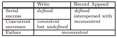
After a sequence of successful mutations, the mutated file region is guaranteed to be defined and contain the data written by the last mutation. GFS achieves this by applying mutations to a chunk in the same order on all its replicas and using chunk version numbers to detect any replica that has become state because it has missed mutations while its chunkserver was down. State replicas will never be involved in mutation or given to clients asking the master for chunk locations.

Since clients cache chunklocations, they may read from a stale replica before that information is refreshed. This window is limited by the cache entry’s timeout and the next open of the file, which purges from the cache all chunkinformation for that file. Moreover, as most of our files are append-only, a stale replica usually returns a premature end of chunkrather than outdated data. When a reader retries and contacts the master, it will immediately get current chunklocations.

Long after a successful mutation, component failures can of course still corrupt or destroy data. GFS identifies failed chunkservers by regular handshakes between master and all chunkservers and detects data corruption by checksumming.

High availability:

Among hundreds of servers in a GFS cluster, some are bound to be unavailable at any given time. We keep the overall system highly available with two simple yet effective strategies: fast recovery and replication.

Fast recovery: Both the master and the chunkserver are designed to restore their state and start in seconds no matter how they terminated. Chunk replication: Each chunk is replicated on multiple chunkservers on different racks. Users can specify different replication levels for different parts of the file namespace. Master replication: The master state is replicated for reliability. Its operations and checkpoints are replicated on multiple machines. A mutation to the state is considered committed only after its log record has been flushed to disk locally and on all master replicas. For simplicity, one master process remains in charge of all mutations as well as background activities such as garbage collection that change the system internally. When it fails, it can restart almost instantly. If its machine or diskfails, monitoring infrastructure outside GFS starts a new master process elsewhere with the replicated operation log. Clients use only the canonical name of the master (e.g. gfs-test), which is a DNS alias that can be changed if the master is relocated to another machine. Moreover shadow masters provide read-only access to the file system even when the primary master is down. They are shadows, not mirrors, in that they may lag the primary slightly, typically fractions of second. They enhance read availability for files that are not being actively mutated or applications that do not ming getting slightly stale results. To keep itself informed, a shadow master reads a replica of the growing operation log and applies the same sequence of changes to its data structures exactly as the primary does. Like the primary, it polls chunkservers at startup (and infrequently thereafter) to locate chunkreplicas and exchanges frequent handshake messages with them to monitor their status. It depends on the primary master only for replica location updates resulting from the primary’s decisions to create and delete replicas.

Data integrity:

Each chunkserver uses checksumming to detect corruption of stored data. Given that a GFS cluster often has thousands of disks on hundreds of machines, it regularly experiences diskfailures that cause data corruption or loss on both the read and write paths. We can recover from corruption using other chunkreplicas, but it would be impractical to detect corruption by comparing replicas across chunkservers. Each chunkserver must independently verify the integrity of its own copy by maintaining checksums.

Limitations:

As the system has grown in usage, problems have emerged with the centralized master scheme:

• Despite the separation of control and data flow and the performance optimization of the master, it is emerging as a bottleneck in the design.
• Despite the reduced amount of metadata stemming from the large chunk size, the amount of metadata stored by each master is increasing to a level where it is difficult to actually keep all metadata in main memory.

Special snapshot operation:

The snapshot operation makes a copy of a file or a directory almost instantaneously, while minimizing any interruptions of ongoing mutations. The users canuse it to quickly create branch copies of huge data sets (and often copies of those copies, recursively), or to checkpoint the current state before experimenting with changes that can later be committed or rolled backeasily.

Like AFS, GFS uses standard copy-on-write techniques to implement snapshots. When the master receives a snapshot request, it first revokes any outstanding leases on the chunks in the files it is about to snapshot. This ensures that any subsequent writes to these chunks will require an interaction with the master to find the lease holder. This will give the master an opportunity to create a new copy of the chunk first.

After the leases have been revoked or have expired, the master logs the operation to disk. It then applies this log record to its in-memory state by duplicating the metadata for the source file or directory tree. The newly created snapshot files point to the same chunks as the source files.

The first time a client wants to write to a chunk C after the snapshot operation, it sends a request to the master to find the current lease holder. The master notices that the reference count for chunk C is greater than one. It defers replying to the client request and instead picks a new chunk handle C’. It then asks each chunkserver that has a current replica of C to create a new chunkcalled C’. By creating the new chunkon the same chunkservers as the original, we ensure that the data can be copied locally, not over the network(our disks are about three times as fast as our 100 Mb Ethernet links). From this point, request handling is no different from that for any chunk: the master grants one of the replicas a lease on the new chunkC’ and replies to the client, which can write the chunknormally, not knowing that it has just been created from an existing chunk.

ok:

so performance and scalability are essentially same:

reliability - replication (hence consistency), high availability (fast recovery), data integrity (error detection and correction)

Chubby

Chubby is a crucial service at the heart of the Google infrastructure offering storage and coordination services for other infrastructure services, including GFS and Bigtable. Chubby is multi-faceted service offering four distinct capabilities:

• It provides coarse-grained distributed locks to synchronize distributed activities in what is a large-scale, asynchronous environment.
• It provides a file system offering the reliable storage of small files (complementing the service offered by GFS).
• It can be used to support the election of a primary in a set of replicas (as needed for example by GFS)
• It is used as a name service within Google.

Interface:

Architecture:

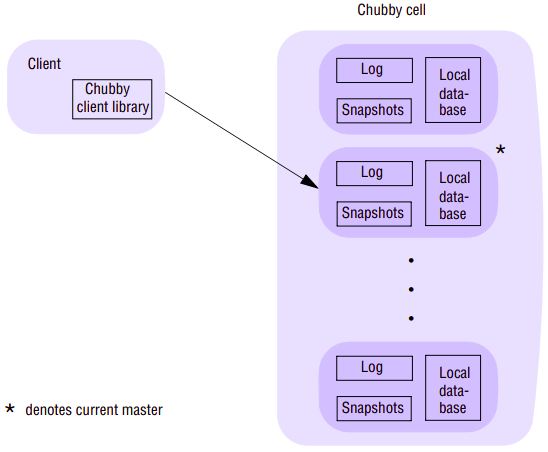
A single instance of a Chubby system is known as a cell; each cell consists of a relatively small number of replicas (typically five) with one designated as master. Client applications access this set of replicas via a Chubby library, which communicates with the remote servers using the RPC service. The replicas are placed at failure-independent sites to minimize the potential for correlated failures – for example, they will not be contained within the same rack. All replicas are typically contained within a given physical cluster, although this is not required for the correct operation of the protocol and experimental cells have been created that span Google data centres.

Each replica maintains a small database whose elements are entities in the Chubby namespace – that is, directories and files/locks. The consistency of the replicated database is achieved using an underlying consensus protocol (an implementation of Lamport’s Paxos algorithm that is based around maintaining operation logs. As logs can become very large over time, Chubby also supports the creation of snapshots - complete views of system state at a given point of time. Once snapshot is taken, previous logs can be deleted with the consistent state of the system at any point determined by the previous snapshot together with the applications of the set of operations in the log.

A Chubby session is a relationship between a client and a Chubby cell. This is maintained using KeepAlive handshakes between the two entities. To improve performance, the Chubby library implements client caching, storing file data, metadata and information on open handles. In contrast to GFS (with its large, sequential reads and appends), client caching is effective in Chubby with its small files that are likely to be accessed repeatedly. Because of this caching, the system must maintain consistency between a file and a cache as well as between the different replicas of the file. The required cache consistency in Chubby is achieved as follows. Whenever a mutation is to occur, the associated operation (for example, SetContents) is blocked until all associated caches are invalidated (for efficiency, the invalidation requests are piggybacked onto KeepAlive replies from the master with the replies sent immediately when an invalidation occurs). Cached data is also never updated directly.

The end result is a very simple protocol for cache consistency that delivers deterministic semantics to Chubby clients. Contrast this with the client caching regime in NFS, for example, where mutations do not result in the immediate updating of cached copies, resulting in potentially different versions of files on different client nodes.

Paxos??

BigTable

GFS offers a system for storing and accessing large flat files whose content is accessed relative to byte offsets within a file, allowing programs to store large quantities of data and perform read and write (especially append) operations optimized for the typical use within the organization. While this is an important building block, it is not sufficient to meet all of Google’s data needs. There is a strong need for a distributed storage system that provides access to data that is indexed in more sophisticated ways related to its content and structure.

Web search and nearly all of the other Google applications, including the crawl infrastructure, Google Earth/Maps, Google Analytics and personalized search, use structured data access. Google Analytics, for example, stores information on raw clicks associated with users visiting a web site in one table and summarizes the analyzed information in a second table.

One choice for Google would be to implement (or reuse) a distributed database, for example a relational database with a full set of relational operators provided (for example, union, selection, projection, intersection and join). But the achievement of good performance and scalability in such distributed databases is recognized as a difficult problem and, crucially, the styles of application offered by Google do not demand this full functionality.

Google therefore has introduced Bigtable, which retains the table model offered by relational databases but with a much simpler interface suitable for the style of application and service offered by Google and also designed to support the efficient storage and retrieval of quite massive structured datasets.

Interface:

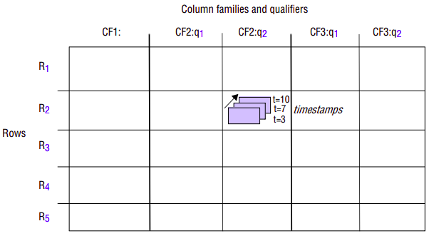
Bigtable is a distributed storage system that supports the storage of potentially vast volumes of structured data. The name is strongly indicative of what it offers, providing storage for what are very big tables (often in the terabyte range). More precisely, Bigtable supports the fault-tolerant storage, creation and deletion of tables where a given table is a three-dimensional structure containing cells indexed by a row key, a column key and a timestamp:

Rows: Each row in a table has an associated row key that is an arbitrary string of up to 64 kilobytes in size, although most keys are significantly smaller. A row key is mapped by Bigtable to the address of a row. A given row contains potentially large amounts of data about a given entity such as a web page. Given that it is common within Google to process information about web pages, it is quite common, for example, for row keys to be URLs with the row then containing information about the resources referenced by the URLs. Bigtable maintains a lexicographic ordering of a given table by row key, and this has some interesting repercussions. When we examine the underlying architecture, subsequences of rows map onto tablets, which are the unit of distribution and placement. Hence it is beneficial to manage locality by assigning row keys that will be close or even adjacent in the lexicographic order. This implies that URLs may make bad key choices, but URLs with the domain portion reversed will provide much stronger locality for data accesses because common domains will be sorted together, supporting domain analyses. To illustrate this, consider information stored on the BBC web site related to sport. If such information is stored under URLs such as www.bbc.co.uk/sports and www.bbc.co.uk/football, then the resultant sort will be rather random and dominated by the lexicographic order of early fields. If, however, it is stored under uk.co.bbc.www/sport and uk.co.bbc.www/football, the related information is likely to be stored in the same tablet. It should be stressed that this key assignment is left entirely to the programmer so they must be aware of this (ordering) property to exploit the system optimally. To deal with concurrency issues, all accesses to rows are atomic (echoing similar design decisions in GFS and Chubby).

Columns: The naming of columns is more structured than that of rows. Columns are organized into a number of column families – logical groupings where the data under a family tends to be of the same type, with individual columns designated by qualifiers within families. In other words, a given column is referred to using the syntax family:qualifier, where family is a printable string and qualifier is an arbitrary string. The intended use is to have a relatively small number of families for a given table but a potentially large number of columns (designated by distinct qualifiers) within a family. This can be used to structure data associated with web pages, with valid families being the contents, any anchors associated with the page and the language that is used in the web page. If a family name refers to just one column it is possible to omit the qualifier. For example, a web page will have one contents field, and this can be referred to using the key name contents:.

Timestamps: Any given cell within Bigtable can also have multiple versions indexed by timestamp, where the timestamp is either related to real time or can be an arbitrary value assigned by the programmer (for example, a logical time, or a version identifier). The various versions are sorted by reverse timestamp with the most recent version available first. This facility can be used, for example, to store different versions of the same data, including the content of web pages, allowing analyses to be carried out over historical data as well as the current data. Tables can be set up to apply garbage collection on older versions automatically, therefore reducing the burden on the programmer to manage the large datasets and associated versions.

Bigtable supports an API that provides a wide range of operations, including:

• the creation and deletion of tables;
• the creation and deletion of column families within tables;
• accessing data from given rows;
• writing or deleting cell values;
• carrying out atomic row mutations including data accesses and associated write and delete operations
• more global, cross-row transactions are not supported
• iterating over different column families, including the use of regular expressions to identify column ranges
• associating metadata such as access control information with tables and column families

Architecture:

A Bigtable is broken up into tablets, with a given tablet being approximately 100–200 megabytes in size. The main tasks of the Bigtable infrastructure are therefore to manage tablets and to support the operations described above for accessing and changing the associated structured data. The implementation also has the task of mapping the tablet structure onto the underlying file system (GFS) and ensuring effective load balancing across the system.

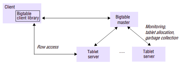
A single instance of a Bigtable implementation is known as a cluster, and each cluster can store a number of tables. The architecture of a Bigtable cluster is similar to that of GFS, consisting of three major components:

• a library component on the client side;
• a master server;
• a potentially large number of tablet servers.

As of 2008, 388 production clusters ran across multiple Google machine clusters, with an average of around 63 tablet servers per cluster but with many being significantly larger (some with more than 500 tablet servers per cluster). The number of tablet servers per cluster is also dynamic, and it is common to add new tablet servers to the system at runtime to increase throughput.

Two of the key design decisions in Bigtable are identical to those made for GFS.

• Firstly, Bigtable adopts a single master approach, for exactly the same reasons – that is, to maintain a centralized view of the state of the system thus supporting optimal placement and load-balancing decisions and because of the inherent simplicity in implementing this approach.
• Secondly, the implementation maintains a strict separation between control and data with a lightweight control regime maintained by the master and data access entirely through appropriate tablet servers, with the master not involved at this stage (to ensure maximum throughput when accessing large datasets by interacting directly with the tablet servers)

In particular, the control tasks associated with the master are as follows:

• monitoring the status of tablet servers and reacting to both the availability of new tablet servers and the failure of existing ones;
• assigning tablets to tablet servers and ensuring effective load balancing;
• garbage collection of the underlying files stored in GFS.

Bigtable goes further than GFS in that the master is not involved in the core task of mapping tablets onto the underlying persistent data (which is stored in GFS). This means that Bigtable clients do not have to communicate with the master at all (compare this with the open operation in GFS, which does involve the master), a design decision that significantly reduces the load on the master and the possibility of the master becoming a bottleneck.

Data storage in Bigtable:

The mapping of tables in Bigtables onto GFS involves several stages:

• A table is split into multiple tablets by dividing the table up by row, taking a row range up to a size of around 100–200 megabytes and mapping this onto a tablet. A given table will therefore consist of multiple tablets depending on its size. As tables grow, extra tablets will be added.
• Each tablet is represented by a storage structure that consists of set of files that store data in a particular format (the SSTable) together with other storage structures implementing logging.
• The mapping from tablets to SSTables is provided by a hierarchical index scheme inspired by B+-trees.

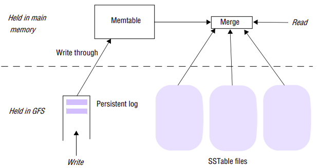
The main unit of storage in Bigtable is the SSTable (a file format that is also used elsewhere in the Google infrastructure). An SSTable is organized as an ordered and immutable map from keys to values, with both being arbitrary strings. Operations are provided to efficiently read the value associated with a given key and to iterate over a set of values in a given key range. The index of an SSTable is written at the end of the SSTable file and read into memory when an SSTable is accessed. This means that a given entry can be read with a single disk read. An entire SSTable can optionally be stored in main memory.

A given tablet is represented by a number of SSTables. Rather than performing mutations directly on SSTables, writes are first committed to a log to support recovery, with the log also held in GFS. The log entries are written through to the memtable held in main memory. The SSTables therefore act as a snapshot of the state of a tablet and, on failure, recovery is implemented by replaying the most recent log entries since the last snapshot. Reads are serviced by providing a merged view of the data from the SSTables combined with the memtable. Different levels of compaction are performed on this data structure to maintain efficient operation. Note that SSTables can also be compressed to reduce the storage requirements of particular tables in Bigtable. Users can specify whether tables are to be compressed and also the compression algorithm to be used.

As mentioned above, the master is not involved in the mapping from tables to stored data. Rather, this is managed by traversing an index based on the concept of B+- trees (a form of B-tree where all the actual data is held in leaf nodes, with other nodes containing indexing data and metadata).

Read in Bigtable:

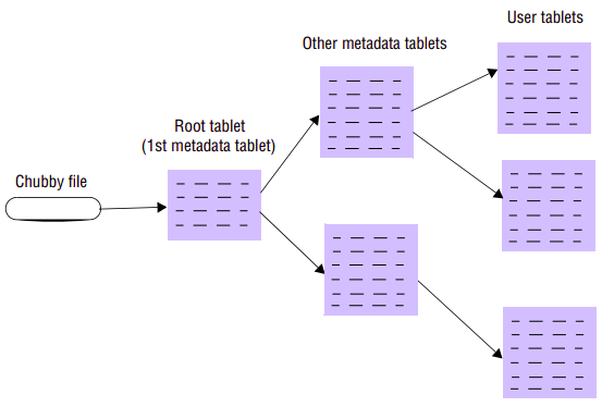
• A Bigtable client seeking the location of a tablet starts the search by looking up a particular file in Chubby that is known to hold the location of a root tablet – that is, a tablet containing the root index of the tree structure.
• This root tablet contains metadata about other tablets – specifically about other metadata tablets, which in turn contain the location of the actual data tablets.
• The root tablet together with the other metadata tablets form a metadata table, with the only distinction being that the entries in the root tablet contain metadata about metadata tablets, which in turn contain metadata about the actual data tablets.

With this scheme, the depth of the tree is limited to three. The entries in the metadata table map portions of tablets onto location information, including information about the storage representation for this tablet (including the set of SSTables and the associated log)

Load balancing:

To assign tablets, the master must map the available tablets in the cluster to appropriate tablet servers. The master has an accurate list of tablet servers that are ready and willing to host tablets and a list of all the tablets associated with the cluster. The master also maintains the current mapping information together with a list of unassigned tablets (which is populated, for example, when a tablet server is removed from the system). By having this global view of the system, the master ensures unassigned tablets are assigned to appropriate tablet servers based on responses to load requests, updating the mapping information accordingly.

Note that a master also has an exclusive lock of its own (the master lock), and if this is lost due to the Chubby session being compromised, the master must terminate itself (again, reusing Chubby to implement additional functionality). This does not stop access to data but rather prevents control operations from proceeding. Bigtable is therefore still available at this stage. When the master restarts, it must retrieve the current status. It does this by first creating a new file and obtaining the exclusive lock ensuring it is the only master in the cluster, and then working through the directory to find tablet servers, requesting information on tablet assignments from the tablet servers and also building a list of all tablets under its responsibility to infer unassigned tablets. The master then proceeds with its normal operation.

(monitoring how? see chubby and bigtable)

Distributed Computation Services

To complement the storage and coordination services, it is also important to support high-performance distributed computation over the large datasets stored in GFS and Bigtable. The Google infrastructure supports distributed computation through the MapReduce service and also the higher-level Sawzall language.

MapReduce

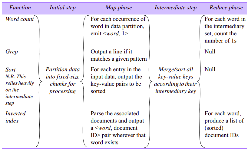
Given the huge datasets in use at Google, it is a strong requirement to be able to carry out distributed computation by breaking up the data into smaller fragments and carrying out analyses of such fragments in parallel, making use of the computational resources offered by the physical architecture of commodity hardware. Such analyses include common tasks such as sorting, searching and constructing inverted indexes (indexes that contain a mapping from words to locations in different files, this being key in implementing search functions). MapReduce is a simple programming model to support the development of such applications, hiding underlying detail from the programmer including details related to the parallelization of the computation, monitoring and recovery from failure, data management and load balancing onto the underlying physical infrastructure.

Interface and Programming Model:

MapReduce allows us to express the simple computations but hides the messy details of parallelization, fault-tolerance, data distribution and load balancing in a library. The key principle behind MapReduce is the recognition that many parallel computations share the same overall pattern - that is:

• break the input data into a number of chunks;
• carry out initial processing on these chunks of data to produce intermediary results;
• combine the intermediary results to produce the final output.

The specification of the associated algorithm can then be expressed in terms of two functions, one to carry out the initial processing and the second to produce the final results from the intermediary values. It is then possible to support multiple styles of computation by providing different implementations of these two functions. Crucially, by factoring out these two functions, the rest of the functionality can be shared across the different computations, thus achieving huge reductions in complexity in constructing such applications.

More specifically, MapReduce specifies a distributed computation in terms of two functions, map and reduce (an approach partially influenced by the design of functional programming languages such as Lisp, which provide functions of the same name, although in functional programming the motivation is not parallel computation):

• The map function, written by user, takes a set of key-value pairs as input and produces a set of intermediary key-value pairs as output.
• The intermediaries are then sorted by key value so that all intermediary results are ordered by intermediary key. This is broken up into groups and passed to reduce instances, also written by user, which carry out their processing to produce a list of values for each group (for some computations, this could be a single value).

The MapReduce implementation is responsible for breaking the data into chunks, creating multiple instances of the map and reduce functions, allocating and activating them on available machines in the physical infrastructure, monitoring the computations for any failures and implementing appropriate recovery strategies, despatching intermediary results and ensuring optimal performance of the whole system.

Programs written in this functional style are automatically parallelized and executed on a large cluster of commodity machines. The run-time system takes care of the details of partitioning the input data, scheduling the program’s execution across a set of machines, handling machine failures, and managing the required inter-machine communication. This allows programmers without any experience with parallel and distributed systems to easily utilize the resources of a large distributed system.

Mappers and reducers:

A part of the design of MapReduce algorithms involves imposing the key-value structure on arbitrary datasets. For a collection of web pages, keys may be URLs and values may be the actual HTML content. For a graph, keys may represent node ids and values may contain the adjacency lists of those nodes. In some algorithms, input keys are not particularly meaningful and are simply ignored during processing, while in other cases input keys are used to uniquely identify a datum (such as a record id). In MapReduce, the programmer defines a mapper and a reducer with the following signatures:

map: $(k_1,v_1)\to \text{list}(k_2,v_2)$ reduce: $(k_2,\text{list}(v_2))\to \text{list}(k_3,v_3)$ The mapper is applied to every key-value pair (split across an arbitrary number of files) to generate an arbitrary number of intermediate key-value pairs. The reducer is applied to all values associated with the same intermediate key to generate output key-value pairs. Implicit between the map and reduce phases is a distributed group-by operation on intermediate keys. Intermediate data arrive at each reducer in order, sorted by the key. However, no ordering relationship is guaranteed for keys across different reducers. Output key-value pairs from each reducer are written persistently back onto the distributed file system (whereas intermediate key-value pairs are transient and not preserved).

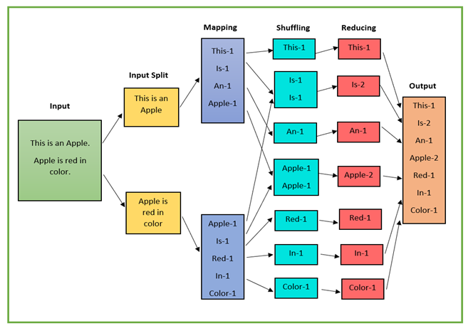
Example: word counting:

Consider the problem of counting the number of occurrences of each word in a large collection of documents. The user would write code similar to the following pseudo-code:

Map:

map(String key, String value): 
	// key: document name 
	// value: document contents 
	for each word w in value: 
		EmitIntermediate(w, "1");

Reduce:

reduce(String key, Iterator values): 
	// key: a word 
	// values: a list of counts
	int result = 0; 
	for each v in values: 
		result += ParseInt(v); 
	Emit(AsString(result));

The map function emits each word plus an associated count of occurrences (just 1 in this example). The reduce function sums together all counts emitted for a particular word. In addition, the user writes code to fill in a mapreduce specification object with the names of the input and output files, and optional tuning parameters. The user then invokes the MapReduce function, passing it the specification object. The user’s code is lined together with the MapReduce (implemented in C++).

Example: web search for ‘distributed systems book’:

Assuming it is supplied with a web page name and its content as input, the map function searches linearly through the contents, emitting a key-value pair consisting of (say) the phrase followed by the name of the web document containing this phrase wherever it finds the strings ‘distributed’ followed by ‘system’ followed by ‘book’ (the example can be extended to also emit a position within the document). The reduce function is in this case is trivial, simply emitting the intermediary results ready to be collated together into a complete index.

Others:

With this approach, it is possible to make significant savings in terms of lines of code by reusing the underlying MapReduce framework. For example, Google reimplemented the main production indexing system in 2003 and reduced the number of lines of C++ code in MapReduce from 3,800 to 700 – a significant reduction, albeit in a relatively small system.

This also results in other key benefits, including making it easier to update algorithms as there is a clean separation of concerns between what is effectively the application logic and the associated management of the distributed computation. . In addition, improvements to the underlying MapReduce implementation immediately benefit all MapReduce applications. The downside is a more prescriptive framework, albeit one that can be customized by specifying the map and reduce and indeed other functions.

Architecture:

MapReduce is implemented by a library that, as mentioned above, hides the details associated with parallelization and distribution and allows the programmer to focus on specifying the map and reduce functions. This library is built on top of other aspects of the Google infrastructure, in particular using RPC for communication and GFS for the storage of intermediary values. It is also common for MapReduce to take its input data from Bigtable and produce a table as a result.

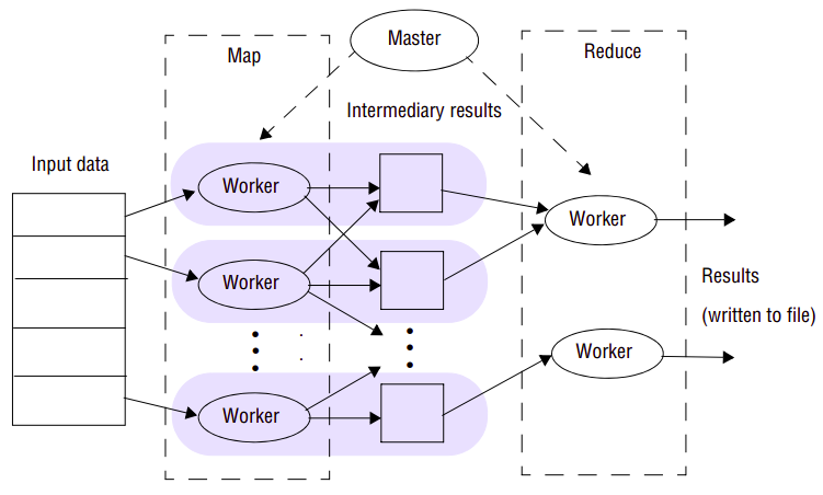
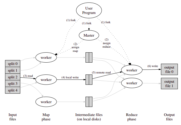
The overall execution of a MapReduce program shows the key phases involved in execution:

• The first stage is to split the input file into M pieces, with each piece being typically 16–64 megabytes in size (therefore no bigger than a single chunk in GFS). The actual size is tunable by the programmer and therefore the programmer is able to optimize this for the particular parallel processing to follow. The key space associated with the intermediary results is also partitioned into R pieces using a (programmable) partition function. The overall computation therefore involves M map executions and R reduce executions.

• The MapReduce library then starts a set of worker machines (workers) from the pool available in the cluster, with one being designated as the master and others being used for executing map or reduce steps. The number of workers is normally much less than M+R. For example, Ghemawat report on typical figures of M=200,000, R=5000 with 2000 worker machines allocated to the task. The goal of the master is to monitor the state of workers and allocate idle workers to tasks, the execution of map or reduce functions. More precisely, the master keeps track of the status of map and reduce tasks in terms of being idle, inprogress or completed and also maintains information on the location of intermediary results for passing to workers allocated a reduce task.

  Segway: A principle on which machine to schedule task: Network bandwidth is relatively scarce resource in our computing environment. We conserve network bandwidth by taking advantage of the fact that the input data is stored on the local disks of the machines that make up our cluster. GFS divides each file into 64 MB blocks, and stores several copies of each block (typically 3 copies) on different machines. The MapReduce master takes the location information of the input files into account and attempts to schedule a map tasks on a machine that contains a replica of the corresponding input data. Failing that, it attempts to schedule a map task near a replica of that task’s input data (e.g. on a worker machine that is on the same network switch as the machine containing the data). When running large MapReduce operations on a significant fraction of the workers in a cluster, most input data is read locally and consumes no network bandwidth.

• A worker that has been assigned a map task will first read the contents of the input file allocated to that map task, extract the key-value pairs and supply them as input to the map function. The output of the map function is a processed set of key/value pairs that are held in an intermediary buffer. As the input data is stored in GFS, the file will be replicated on (say) three machines. The master attempts to allocate a worker on one of these three machines to ensure locality and minimize the use of network bandwidth. If this is not possible, a machine near the data will be selected.

• The intermediary buffers are periodically written to a file local (not global GFS) to the map computation. At this stage, the data are partitioned according to the partition function, resulting in R regions. This partition function, which is crucial to the operation of MapReduce, can be specified by the programmer, but the default is to perform a hash function on the key and then apply modulo R to the hashed value to produce R partitions, with the end result that intermediary results are grouped according to the hash value. Ghemawat provide alternative example where keys are URLs and the programmer wants to group intermediary results by the associated host: hash(Hostname(key)) mod R. The master is notified when partitioning has completed and is then able to request the execution of associated reduce functions.

• When a worker is assigned to carry out a reduce function, it reads its corresponding partition from the local disk of the map workers using RPC. This data is sorted by the MapReduce library ready for processing by the reduce function. Once sorting is completed, the reduce worker steps through the keyvalue pairs in the partition applying the reduce function to produce an accumulated result set, which is then written to an output file. This continues until all keys in the partition are processed.

• After successful completion, the output of the mapreduce execution is available in the R output files (one per reduce task, with files names as specified by the user). Typically, users do not need to combine these R output files into one file – they often pass these files as input to another MapReduce call, or use them from another distributed application that is able to deal with input that is partitioned into multiple files.

Fault Tolerance:

The MapReduce implementation provides a strong level of fault tolerance, in particular guaranteeing that if the map and reduce operations are deterministic with respect to their inputs (that is they always produce the same outputs for a given set of inputs), then the overall MapReduce task will produce the same output as a sequential execution of the program, even in the face of failures.

Worker failure:

To deal with failure, the master sends a ping message periodically to check that a worker is alive and carrying out its intended operation. If no response is received, it is assumed that the worker has failed and this is recorded by the master. The subsequent action then depends on whether the task executing was a map or a reduce task:

• If the worker was executing a map task, this task is marked idle, implying it will be rescheduled. This happens irrespective of whether the associated task is in progress or completed. Remember that results are stored on local disks, and hence if the machine has failed the results will be inaccessible.
• If the worker was executing a reduce task, this task is marked as idle only if it was still in progress; if it is completed, the results will be available as they are written to the global (and replicated) file system.

Note that to achieve the desired semantics, it is important that the outputs from map and reduce tasks are written atomically, a property ensured by the MapReduce library in cooperation with the underlying file system.

MapReduce also implements a strategy to deal with workers that may be taking a long time to complete (known as stragglers). Google has observed that it is relatively common for some workers to run slowly, for example because of a faulty disk that may perform badly due to a number of error-correction steps involved in data transfers. To deal with this, when a program execution is close to completion, the master routinely starts backup workers for all remaining in-progress tasks. The associated tasks are marked as completed when either the original or the new worker completes. This is reported as having a significant impact on completion times, again circumventing the problem of working with commodity machines that can and do fail.

Master failure:

The master keeps several data structures. For each map and reduce task, it stores the state (idle, in-progress, or completed), and the identify of the worker machines (for non-idle tasks). The master is the conduit through which the location of intermediate file regions is propagated from map tasks to reduce tasks. Therefore, for each completed map tasks, the master stores the locations and sizes of the R intermediate file regions produced by the map task. Updates to this location and size information are received as map tasks are completed. The information is pushed incrementally to workers that have in-progress reduce tasks.

Refinements

• Custom partitioners and combiners
• Status information

In some cases, there is significant repetition in the intermediate keys produced by each map task, and the user specified Reduce function is commutative and associative. A good example of this is the word counting example. Since word frequencies tend to follow a Zipf distribution, each map task will produce hundreds or thousands of records of the form <the, 1>. All of these counts will be sent over the network to a single reduce task and then added together by the Reduce function to produce one number. We allow the user to specify an optional Combiner function that does partial merging of this data before it is sent over the network. The Combiner function is executed on each machine that performs a map task. Typically the same code is used to implement both the combiner and the reduce functions. The only difference between a reduce function and a combiner function is how the MapReduce library handles the output of the function. The output of a reduce function is written to the final output file. The output of a combiner function is written to an intermediate file that will be sent to a reduce task.

(see sawzall, addition to mapreduce, as well)

NoSQL

NoSQL is an approach to database design that focuses on providing a mechanism for storage and retrieval of data that is modeled in means other than the tabular relations used in relational databases. Instead of the typical tabular structure of a relational database, NoSQL databases house data within one data structure. Since this non-relational database design does not require a schema, it offers rapid scalability to manage large and typically unstructured data sets. NoSQL systems are sometimes called Not only SQL to emphasize that they may support SQL-like query languages or sit alongside SQL databases in polyglot-persistent architectures.

Features:

• Motivations for this approach include simplicity of design, simpler horizontal scaling to clusters of machines, finer control over availability, and limiting the object-relational impedance mismatch.

• The data structures used in NoSQL databases (e.g. key-value pair, wide column, graph, or document) are different from those used by default in relational databases, making some operations faster in NoSQL.

• Many NoSQL stores compromise consistency (in the sense of CAP theorem) in favor of availability, partition tolerance, and speed.

• Barriers to the greater adoption of NoSQL stores include the use of low-level query languages (instead of SQL, for instance), lack of ability to perform ad hoc joins across tables, lack of standardized interface, and huge previous investments in existing relational databases.

• Instead, most NoSQL databases offer a concept of eventual consistency, in which database changes are propagated to all nodes eventually (typically within milliseconds), so queries for data might not return updated data immediately or might result in reading data that is not accurate, a problem known as stale read.

Types and examples:

There are various ways to classify NoSQL databases, with different categories and subcategories, some of which overlap.

Key-value store

uses the associative array (also called a map or dictionary) as their fundamental data model. In this model, data is represented as a collection of key-value pairs, such that each possible key appears at most once in the collection. Dictionaries contain a collection of objects, or records, which in turn have many different fields, within them, each containing data. These records are stored and retrieved using a key that uniquely identifies the record, and is used to find the data within the database.

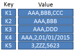
Example: DynamoDB, Couchbase

Document store

The central concept of a document-oriented database is the notion of a document. While each document-oriented database implementation differs on the details of this definition, in general, they all assume documents encapsulate and encode data (or information) in some standard format or encoding. Encodings in use include XML, YAML, JSON, as well as binary forms like BSON.

Document databases contrast strongly with the traditional database (RDB). Relational databases generally store data in separate tables that are defined by the programmer, and a single object may be spread across several tables. Document databases store all information for a given object in a single instance in the database, and every stored object can be different from every other.

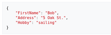
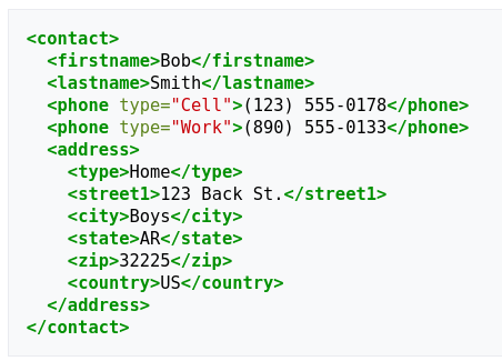
Example: MongoDB

Graph

Graph databases are designed for data whose relations are well represented as a graph consisting of elements connected by a finite number of relations.  Examples of data include social relations, public transport links, road maps, network topologies, etc. A labeled-property graph model is represented by a set of nodes, relationships, properties, and labels. Both nodes of data and their relationships are named and can store properties represented by key value pairs.

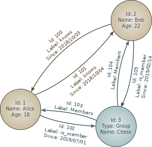
Example: ArangoDB, RedisGraph

Triplestore? A triplestore is a purpose-built database for the storage and retrieval of triples through semantic queries. A triple is data entity composed of subject-predicate-object, like “Bob is 35” or “Bob knows Fred”.

Column-oriented store

The columnar DBMS stores tables by column rather than by row. Benefits include more efficient access to data when only querying a subset of columns (by eliminating the need to read columns that are not relevant), and more options for data compression. However, they are typically less efficient for inserting new data.

Practical use of a column store store versus a row store differs little in the relational DBMS world. Both columnar and row databases can use traditional database query languages like SQL to load data and perform queries. Both row and columnar databases can become the backbone in a system to serve data for common ETL and tools.

A relational DBMS provides data that represents a 2D table of columns and rows. For example, a database might have this:

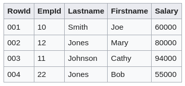
In an actual implementation, storage hardware requires the data to be serialized into one form or another. The most expensive operations involving hard disks are seeks. In order to improve overall performance, related data should be stored in a fashion to minimize the number of seeks.

A common method of storing a table is to serialize each row of data, like this:

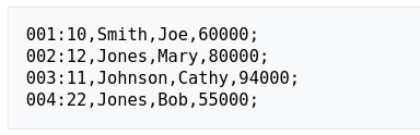
As data is inserted into the table, it is assigned an internal ID, the rowid that is used internally in the system to refer to data. In this case the records has sequential rowid’s independent of user assigned empid. In this example, the DBMS uses short integers to store rowids, in practice, large numbers, 64-bit or 128-bit, are normally used.

Row-oriented systems are designed to efficiently return data for an entire row, or record, in as few operations as possible. This matches the common use-case where the system is attempting to retrieve information about a particular object, say the contact information for a user, or product information for an online shopping system. By storing the record’s data in a single block on the disk, along with related records, the system can quickly retrieve records with a minimum of disk operations.

Row-oriented systems are not efficient at performing set-wide operations on the whole table, as opposed to a small number of specific records. For instance, in order to find all records in the example table with salaries between 40,000 and 50,000, the DBMS would have to fully scan through the entire table looking for matching records.

To improve the performance of these sort of operations, most DBMSs support the use of database indexes, which store all the values from a set of columns along with rowid pointers back into the original table. An index on the salary column would look something like:

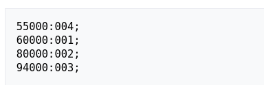
As they store only single pieces of data, rather than entire rows, indexes are generally much smaller than the main table stores. Scanning this smaller set of data reduces the number of disk operations. If the index is heavily used, it can dramatically reduce the time for common operations. The main reason why indexes dramatically improve performance on large datasets is that database indexes on one or more columns are typically sorted by value, which makes range queries operations very fast.

However, maintaining indexes adds overhead to the system, especially when new data is written to the database. Records not only need to be stored in the main table, but any attached indexes have to be updated as well.

A column-oriented database serializes all of the values of a column together, then the values of the next column, and so on. For our example table, the data would be stored in this fashion:

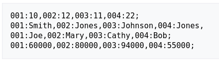
In this layout, any one of the columns more closely matches the structure of an index in a row-oriented system. This may cause confusion that can lead to the mistaken belief a column-oriented store is really just a row-store with an index on every column. However, it is the mapping of the data that differs dramatically. In a row-oriented system, indices map column values to rowids, whereas in a column-oriented system, columns map rowids to column values.

A row-oriented system can retrieve the row in a single disk read, whereas numerous disk operations to collect data from multiple columns are required from a columnar database. However, these whole-row operations are generally rare. In the majority of cases, only a limited subset of data is retrieved. For instance, collecting the first and last names from many rows to build a list of contacts is far more common than reading all data for any single address

Note: A wide-column store can be interpreted as a two-dimensional key-value store. Google’s Bigtable is one of prototypical examples.

CAP Theorem

The CAP theorem, states that any distributed data store can provide any two of the following three guarantees:

Consistency: Every read receives the most recent write or an error. All clients see the same data at the same time, no matter which node they connect to.

Availability: Every request receives a (non-error) message, without the guarantee that it contains the most recent write

Partition tolerance: The system continues to operate despite an arbitrary number of messages being dropped (or delayed) by the network between nodes

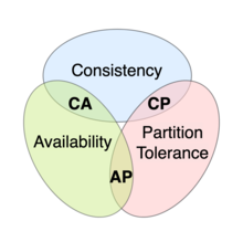
Explanation: No distributed system is safe from network failures, thus partitioning generally has to be tolerated. In the presence of partition, one is then left with two options: consistency or availability. When choosing consistency over availability, the system will return an error or a time out if particular information cannot be guaranteed to be up to date due to network partitioning. When choosing availability over consistency, the system will always process the query and try to return the most recent available version of the information, even if it cannot guarantee it is up to date due to network partitioning.

(The C of CAP is not same as C of ACID)

Proof (somehow):

Let’s consider a very simple distributed system. Our system is composed of two servers, $G_1$ and $G_2$. Both of these servers are keeping track of the same variable, $v$, whose value is initially $v_0$. $G_1$ and $G_2$ can communicate with each other and can also communicate with external clients. Here’s what our system looks like.

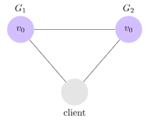
The first thing we do is partition our system. It looks like this.

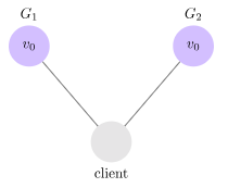
Next, we have our client request that $v_1$ be written to $G_1$. Since our system is available, $G_1$ must respond. Since the network is partitioned, however, $G_1$ cannot replicate its data to $G_2$.

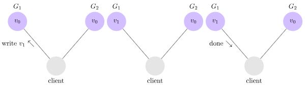
Next, we have our client issue a read request to $G_2$. Again, since our system is available, $G_2$ must respond. And since the network is partitioned, $G_2$ cannot update its value from $G_1$. It returns $v_0$. This is inconsistent.

in NoSQL realm:

MongoDB and the CAP theorem:

MongoDB is a popular NoSQL DBMS that stores data as BSON documents. Relative to CAP theorem, MongoDB is a CP data store - it resolves network partitions by maintaining consistency, while compromising on availability. MongoDB is a single-master system—each replica set can have only one primary node that receives all the write operations. All other nodes in the same replica set are secondary nodes that replicate the primary node’s operation log and apply it to their own data set. By default, clients also read from the primary node, but they can also specify a read preference that allows them to read from secondary nodes. When the primary node becomes unavailable, the secondary node with the most recent operation log will be elected as the new primary node. Once all the other secondary nodes catch up with the new master, the cluster becomes available again. As clients can’t make any write requests during this interval, the data remains consistent across the entire network.

Cassandra and the CAP theorem:

Apache Cassandra is an open source NoSQL database maintained by the Apache Software Foundation. It’s a wide-column database that lets you store data on a distributed network. However, unlike MongoDB, Cassandra has a masterless architecture, and as a result, it has multiple points of failure, rather than a single one. Relative to the CAP theorem, Cassandra is an AP database—it delivers availability and partition tolerance but can’t deliver consistency all the time. Because Cassandra doesn’t have a master node, all the nodes must be available continuously. However, Cassandra provides eventual consistency by allowing clients to write to any nodes at any time and reconciling inconsistencies as quickly as possible. As data only becomes inconsistent in the case of a network partition and inconsistencies are quickly resolved, Cassandra offers repair functionality to help nodes catch up with their peers. However, constant availability results in a highly performant system that might be worth the trade-off in many cases.

HBase and the CAP theorem (not sure):

Apache HBase is an open-source, distributed NoSQL database that is part of the Apache Hadoop ecosystem. It is designed to store large amounts of sparse data in a tabular format and is modeled after Google’s Bigtable. HBase operates on top of the Hadoop Distributed File System (HDFS) and provides Bigtable-like capabilities for Hadoop. Concerning the CAP theorem, HBase is generally considered a CP data store - it prioritizes consistency and partition tolerance over availability. HBase is a master-slave system—there is a master server that handles metadata operations and region server assignments, but the actual data is stored in region servers. The master server is not a bottleneck or single point of failure because region servers can continue to serve read and write requests even if the master is down. However, certain operations like creating or deleting tables, cannot be performed without the master.

MongoDB

MongoDB is cross-platform, document-oriented database program. Classified as a NoSQL database product, MangoDB utilizes JSON-like documents with optional schema. Main features include:

(see from user side here:) MongoDB

Ad-hoc queries: supports field, range query and regular-expression searches. Queries can return specific fields of documents and also include user-defined JavaScript functions.

Indexing: Fields in MongoDB document can be indexed with primary and secondary indices.

Replication: MongoDB provides high availability with replica sets. A replica set consists of two or more copies of the data. Each replica-set member may act in the role of primary or secondary replica at a time. All writes and reads are done on the primary replica by default. Secondary replicas maintain a copy of the data of the primary using built-in replication. When a primary replica fails, the replica set automatically conducts an election process to determine which secondary should become the primary. Secondaries can optionally serve read operations, but that data is only eventually consistent by default. If the replicated MongoDB deployment only has a single secondary member, a separate daemon called an arbiter must be added to the set. It has the single responsibility of resolving the election of the new primary. As a consequence, an ideal distributed MongoDB deployment requires at least three separate servers, even in the case of just one primary and one secondary.

(from docs) A replica set is a group of mongod instances that maintain the same data set. A replica set contains several data bearing nodes and optionally one arbiter node. Of the data bearing node, one and only one member is deemed the primary node, while the other nodes are deemed secondary nodes.

The primary nodes receives all write operations. A replica set can have only one primary capable of confirming write with {w: "majority"} write concern; although in some circumstances, another mongod instances may transiently believe itself to also be primary. The primary records all changes to its data sets in its operation log. i.e oplog.

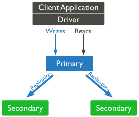
The secondaries replicate the primary’s oplog and apply the operations to their data sets such that the secondaries’ data sets reflect the primary’s data set. If the primary is unavailable, an eligible secondary will hold an election to elect itself the new primary.

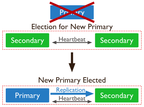
Load balancing: MongoDB scales horizontally using sharding. The user chooses a shard key, which determines how the data in a collection will be distributed. The data is split into ranges (based on the shard key) and distributed across multiple shards, which are masters with one or more replicas. Alternatively, the shard key can be hashed to a map to a shard - enabling an even more data distribution. MongoDB can run over multiple servers, balancing the load or duplicating data to keep the system functional in case of hardware failure.

(from docs)

Sharding is a method for distribution data across multiple machines. MongoDB uses sharding to support deployments with very large data sets and high throughput operations. Database systems with large data sets or high throughput applications can challenge the capacity of a single server. There are two methods for addressing system growth: vertical and horizontal scaling.

Vertical Scaling involves increasing the capacity of a single server, such as using a more powerful CPU, adding more RAM, or increasing the amount of storage space. Limitations in available technology may restrict a single machine from being sufficiently powerful for a given workload. Additionally, Cloud-based providers have hard ceilings based on available hardware configurations. As a result, there is a practical maximum for vertical scaling.

Horizontal Scaling involves dividing the system dataset and load over multiple servers, adding additional servers to increase capacity as required. While the overall speed or capacity of a single machine may not be high, each machine handles a subset of the overall workload, potentially providing better efficiency than a single high-speed high-capacity server. Expanding the capacity of the deployment only requires adding additional servers as needed, which can be a lower overall cost than high-end hardware for a single machine.

MongoDB supports horizontal scaling through sharding.

A MongoDB sharded cluster consists of following components:

• shard: Each shard contains a subset of the sharded data. Each shard must be deployed as a replica set.
• mongos: The mongos acts as a query router, providing an interface between client applications and the sharded cluster.
• config servers: Config servers store metadata and configurations settings for the cluster.

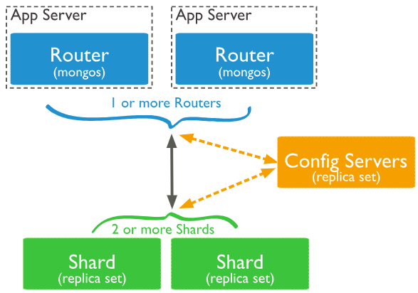
MongoDB uses the shard key to distributed the collection’s documents across shards. The shard key consists of a filed or a multiple fields in the documents. Documents in sharded collections can be missing the shard key fields. Missing shard key fields are treated as having null values when distributing the documents across shards but not when routing queries.

Aggregation: MongoDB provides three ways to perform aggregation: the aggregation pipeline, the map-reduce function and single-purpose aggregation methods. Map-reduce can be used for batch processing of data and aggregation operations. However, according to MongoDB’s documentation, the aggregation pipeline provides better performance for most aggregation operations. The aggregation framework enables users to obtain results similar to those returned by queries that include the SQL GROUP BY clause.

HBase

HBase is a open source non-relational distributed database modeled after Google’s Bigtable and written in Java. It is developed as part of Apache’s Hadoop project and runs on top of HDFS, providing Bigtable-like capabilities for Hadoop. That is, it provides a fault-tolerant way of storing large quantities of sparse data (small amounts of information caught within a large collection of empty or unimportant data, such as finding the 50 largest items in a gorup of 2 billion records, or finding the non-zero items representing less that 0.1% of a huge collection.)

(same as big table lol)

Bigtable Term	HBase Equivalent
Table	Table
Row Key	Row Key
Column Family	Column Family
Column (Qualifier)	Column (Qualifier)
Cell	Cell
Timestamp	Timestamp
Tablets	Regions
Tablet Server	RegionServer
Master Server	HMaster
SSTable	HFile
MemTable	MemStore
Chubby	ZooKeeper
Garbage Collection	Garbage Collection
Compression	Compression
API Operations	API Operations
Transclude of HBase+Architecture.avif

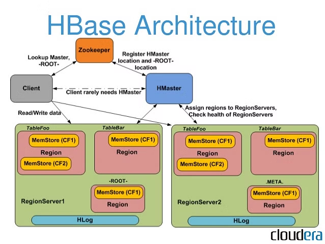
CRUD in HBase:

Operation	Shell Command
Create	create 'myTable', 'cf'
Read	get 'myTable', 'row1'
Update	put 'myTable', 'row1', 'cf:col1', 'newValue'
Delete	delete 'myTable', 'row1', 'cf:col1'
Zookeeper:

(same as chubby)

Chubby Term/Concept	ZooKeeper Equivalent
Cell	Ensemble/Cluster
Replicas	Followers and Observers
Master	Leader
RPC service	Client-Server Communication
Namespace (directories and files/locks)	Znodes
Consensus Protocol (Paxos)	Zab (ZooKeeper Atomic Broadcast)
Snapshots	Snapshots
Sessions	Sessions
Client Caching	Client Caching
Cache Invalidation	Watches (for cache invalidation)
KeepAlive Handshakes	Heartbeats

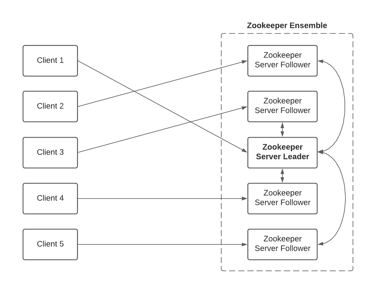Zab:

ZooKeeper Atomic Broadcast (ZAB) is a consensus protocol used by Apache ZooKeeper, inspired by Leslie Lamport’s Paxos algorithm. It ensures distributed consensus by electing a leader to serialize write requests and replicate these to all nodes, maintaining consistent state across the cluster. Simplifying Paxos principles for ZooKeeper’s needs, ZAB is optimized for leader election and consistent transaction ordering, essential for ZooKeeper’s role in distributed coordination.

Cassandra

(hamro siides sararara)

LUCENE

Apache Lucene is an open source Java-based search library providing Application Programming Interfaces for performing common search and search related tasks like indexing, querying, highlighting, language analysis and many others. Lucene is written and maintained by a group of contributers and committers of the Apache Software Foundation. Today, Lucene enjoys widespread adoption powering search on many of today’s most popular websites, applications and devices, such as Twitter, Netflix and Instagram, as well as many other search-based applications.

The main capabilities of Lucene are centered on the creation, maintenance and accessibility of the Lucene inverted index. Lucene consists of a number of features that can be broken down into four main categories:

• analysis of incoming content and queries
• indexing and storage
• searching
• ancillary modules (everything else)

The first three items contribute to what is commonly referred to as the core of Lucene, while the last consists of code libraries that have proven to be useful in solving search-related problems (e.g. result highlighting.)

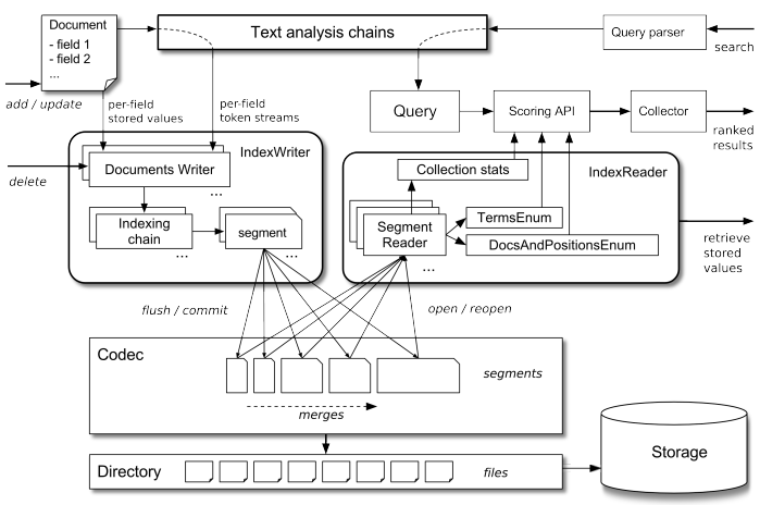
Language analysis:

The analysis capabilities in Lucene are responsible for taking in content in the form of documents to be indexed or queries to be searched and converting them into an appropriate internal representation that can then be used as needed. At indexing time, analysis creates tokens that are ultimately inserted into Lucene’s inverted index, while at query time, tokens are created to help form appropriate query representations. The analysis process consists of three tasks which are chained together to operate on incoming content:

• optional character filtering and normalization (e.g. removing diacritics)
• tokenization
• token filtering (e.g. stemming, lemmatization, stopword removal)

Indexing:

Lucene uses the well-known inverted index representation, with additional functionality for keeping adjacent non-inverted data on a per-document basis. Both in-flight and persistent data uses variety of encoding schemas that affect the size of the index and the cost of the data compression. Lucene uses pluggable mechanisms for data coding and for the actual storage of index data. Incremental updates are supported and stored in index extents (referred to as segments) that are periodically merged into larger segments that minimize the total number of index parts.

1. Document modelling and types: Documents are modeled in Lucene as a flat ordered list of fields with content. Fields have name, content data, float weight (used later for scoring), and other attributes, depending on their type, which together determine how the content is processed and represented in the index. There can be multiple fields with the same name in a document, in which case they will be processed sequentially. Documents are not required to have a unique identifier (though they often carry a field with this role for application-level unique key lookup) - in the process of indexing documents are assigned internal integer identifiers. There are two types of fields: indexed and stored. Indexed fields are analyzed and inverted for searching, while stored fields are stored-as-is for retrieval.

- Field: Title (Indexed)
	  - Name: "title"
	  - Content Data: "Introduction to Lucene"
	  - Weight: 1.0

- Field: Content (Indexed)
	  - Name: "content"
	  - Content Data: "Lucene is a powerful open-source search library written in Java."
	  - Weight: 1.0

- Field: Date (Stored)
	  - Name: "date"
	  - Content Data: "2024-04-03"
	  - Weight: 1.0

- Field: Author (Stored)
	  - Name: "author"
	  - Content Data: "John Doe"
	  - Weight: 1.0

2. Text analysis: The text analysis process generates a sequence of tokens from the input data in a field. These toekns are represented by various attributes, including the main term value and additional metadata like position, offsets, token type, and payload data. The analysis chain comprises character filters, tokenizers, and token filters, which manipulate the token stream. Lucene offers numerous character filters, tokenization strategies, and token filters, supporting multiple languages and specialized functions such as pattern-based tokenization, numeric range searching, stemming, stop word removal, and n-gram creation. This flexibility allows for the creation of intricate text analysis pipelines tailored to specific requirements.

Title:
Tokens: [Introduction, to, Lucene]

Content:
Tokens: [Lucene, is, a, powerful, open-source, search, library, written, in, Java]

3. Indexing chain: The resulting token stream is finally processed by the indexing chain and the supported attributes (term value, position, offsets and payload data) are added to the respective posting lists for each term. Also at this stage documents are assigned their internal document identifiers, which are small sequential integers (for efficient delta compression). These identifiers are ephemeral - they are used for identifying document data within a particular segment, so they naturally change after two or more segments are merged (during index compaction).

Term vectors:

For a DOC-ID doc1:

	Title:
	
	- Term: "Introduction"
	    - Frequency: 1
	    - Positions: [0]
	    - Offsets: [(0, 12)]
	- Term: "to"
	    - Frequency: 1
	    - Positions: [1]
	    - Offsets: [(13, 15)]
	- Term: "Lucene"
	    - Frequency: 1
	    - Positions: [2]
	    - Offsets: [(16, 22)]
	
	Content: ...

For another DOC-ID doc2: ...

Posting lists:

Term: "Introduction"
	- Posting List: [doc1, doc2]
Term: "Introduction"
    - Posting List: [doc1, ...]
Term: "to"
    - Posting List: [doc1]
Term: "Lucene"
    - Posting List: [doc1, doc2, doc3, ...]

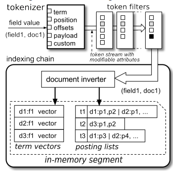
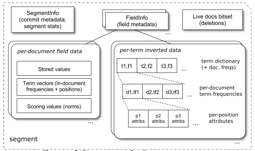
4. Incremental index updates: Indexes can be updated incrementally on-line, simultaneously with searching, by adding new documents and/or deleting existing ones. When new documents are submitted for indexing, their fields undergo the process described in the previous section, and the resulting inverted and non-inverted data is accumulated in new inmemory index extents called “segments”, using a compact in-memory representation. Periodically these in-memory segments are flushed to a persistent storage whenever they reach a configurable threshold - for example, the total number of documents, or the size in bytes of the segment.

Searching:

Lucene’s primary searching concerns can be broken down into a few key areas:

• Lucene’s query model
• Query evaluation
• Scoring
• Common search extensions

1. Query modelling and types: Lucene does not enforce a particular query language: instead it uses Query objects to perform searches. Several Queries are provided as building blocks to express complex queries, and developers can construct their own programmatically or via a Query Parser. Query types provided in Lucene include:

   • term queries that evaluate a single term in a specific field
   • boolean queries supporting AND, OR and NOT where clauses can be any other query
   • proximity queries
   • position-based queries
   • fuzzy and regular expression queries
   • disjunction-max queries and so on This large collection of predefined queries allows developers to express complex criteria for matching and scoring of documents, in a well-structured tree of query clauses

2. Query evaluation: When a Query is executed, each inverted index segment is processed sequentially for efficiency: it is not necessary to operate on a merged view of the postings lists. For each index segment, the Query generates a Scorer: essentially an enumerator over the matching documents with an additional score() method. Finally, a Collector is responsible for actually consuming these Scorers and doing something with the results: for example populating a priority queue of the top-N documents.

3. Scoring: Lucene provides several similarity implementations that offer well-known scoring models: TF/IDF with several different normalizations. The TF-IDF scoring is a statistical method used in information retrieval to evaluate the importance of a term within a document relative to a collection of documents:

   • Term Frequency: TF measures how frequently a term occurs in a document. It is calculated as the ratio of the number of times a term appears in a document to the total number of terms in that document. Lucene uses a vector space model to represent each document as a vector, where each dimension corresponds to a unique term and the value of each dimension represents the TF of the corresponding term in the document.
   • Inverse Document Frequency: IDF measures the rarity of a term across the entire document collection. It is calculated as the logarithm of the ratio of the total number of documents in the collection to the number of documents containing the term.
   • The TF-IDF score of a term in a document is calculated by multiplying its TF value by its IDF value. A high TF-IDF score indicates that the term is both frequent within the document and rare across the collection, making it highly relevant to that document. Documents with higher TF-IDF scores for a particular term are considered more relevant to a search query containing that term.

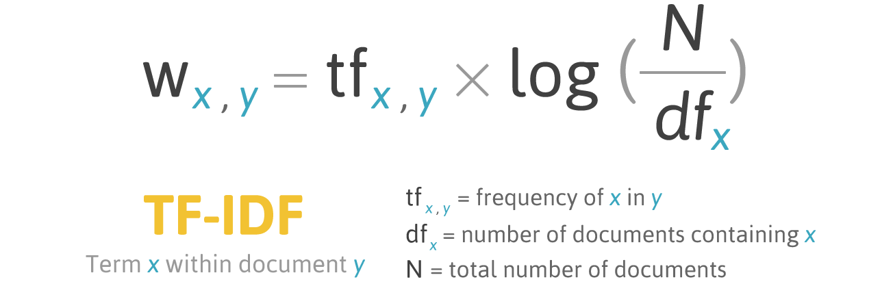
Elastic Search

Elasticsearch is an open-source, distributed search engine built on top of Apache Lucene. It extends Lucene’s capabilities to make it easier to deploy and manage as a standalone system. A node is a single instance of Elasticsearch running on a machine (physical or virtual). Nodes contain shards, and each Elasticsearch cluster can have multiple nodes. A shard in Elasticsearch is essentially a subset of your dataset and functions as a fully operational search engine in its own right. There are two types of shards:

• Primary Shard: Where each document in your dataset is stored initially.
• Replica Shard: Copies of primary shards that provide redundancy and increase fault tolerance, ensuring data is not lost if a primary shard fails and improving query performance by distributing the search load.

Within an Elasticsearch cluster, one node is designated as the master node. This node is responsible for managing the cluster’s overall operation, such as keeping track of which nodes are part of the cluster and deciding where to allocate shards. Although there is one master node at any given time, any node has the potential to be elected as the master, ensuring the cluster can continue operating if the current master fails.

When a request is made to the Elasticsearch cluster, it can be sent to any node. The node that receives the request becomes the coordinating node for that request. Its job is to understand where the relevant data resides within the cluster and route the request appropriately to the correct shard(s) for processing. To distribute the load evenly across the cluster, it may use a method like round-robin for routing requests.

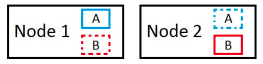There is a single primary and replica on each of the nodes. A client issues an indexing request to node 1 which is then the coordinating node. Node 1 determines that the document should belong to the primary shard hosted on node 2. The request is handed over to the responsible primary shard after being routed to node 2. The primary shard coordinates the indexing with its replica on node 1. When the primary node determines that both shards has indexed the document it responds to node 2, which will route the response back to node 1. Ultimately, node 1 can respond to entire request.

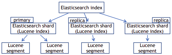
Query language:

There are two kinds of queries: full-text and exact-value. Full-text analyses the entire document and retrieves results based on relevance. Exact-value functions more like an SQL query where the user specifies which fields should have a certain value. Elasticsearch features its own query domain specific language, which is based on the JSON format.

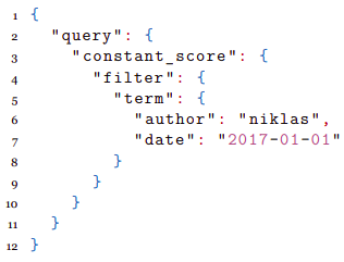
Hadoop

(this is from AWS course, check it AWS Data Pipeline Course)

Apache Hadoop:

Hadoop is an open source framework that uses a distributed processing architecture. Hadoop maps tasks to a cluster of commodity servers for processing. Hadoop consists of four main components:

• Hadoop Distributed File System (HDFS);
• Yet Another Resource Negotiator (YARN);
• MapReduce; and
• Hadoop Common. Hadoop clusters consist of main nodes and worker nodes. In this format, main nodes are responsible for orchestrating jobs, while worker nodes are responsible for processing those jobs.

Benefits:

With Hadoop, you can store as much data as you like. You aren’t required to preprocess data prior to storing it; therefore, the framework provides increased flexibility. Hadoop also has a high degree of fault tolerance, thanks to node failover. If a node fails within a cluster, its tasks are redistributed throughout the other nodes within the cluster. Data loss is likewise prevented by having multiple copies of the same data stored throughout the cluster.

The Hadoop infrastructure is scalable as data processing and computing requirements grow, you can easily add nodes to support that growth in volume and velocity. Because it is an open source framework, Hadoop is free and capable of running on inexpensive hardware. Finally, you can use Hadoop to process structured, unstructured, and semistructured data. You can transform the data into a variety of other formats to integrate with your existing datasets, and you can store the data with or without a schema.

Challenges:

The framework does have a few challenges. Because of its open source nature, stability issues can arise as the framework is updated. You can avoid this challenge by running only the latest stable version. Hadoop also makes heavy use of the Java programming language a commonly targeted language that can leave the framework open to vulnerabilities. Lastly, security concerns are inherent to Hadoop. Lack of authentication and encryption can lead to questions about the veracity of the data.

Hadoop Distributed File System:

The Hadoop Distributed File System, or HDFS, is the distributed file system of the Hadoop framework. You can use HDFS to store huge amounts of data for further processing. HDFS and the Hadoop cluster use a hierarchical node architecture, which consists of a single NameNode that manages multiple DataNodes across clusters.

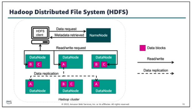
HDFS is typically used by applications that have large datasets, so it’s designed to provide high aggregate data bandwidth. To support data velocity while storing data, HDFS splits the data into small blocks - called data blocks - and stores those blocks across several nodes of the cluster. In the example, a large data file has been split into three data blocks.

Each block resides in a different data node when possible. To avoid losing data if a cluster node fails, HDFS replicates each block several times across different nodes. This enables a high degree of fault tolerance within HDFS. The number of times that a block is replicated is called the replication factor, and it’s a configurable setting. The cluster’s NameNode catalogs the metadata about each file that is stored in the cluster. The cluster DataNodes store the data blocks for each file that has been saved to HDFS.

A Hadoop instance is divided into HDFS and MapReduce. HDFS is used for storing the data and MapReduce is used for processing data. HDFS has five services as follows:

• Name Node
• Secondary Name Node
• Job Tracker
• Data Node
• Task Tracker

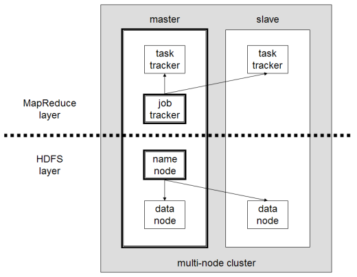
Top three are master services/daemons and bottom two are slave services. Master services can communicate with each other and in the same way slave services can communicate with each other. Name node is a master node and data node is its corresponding slave node and can talk with each other.

• Name Node: HDFS consists of only one Name Node that is called the Master Node. The master node can track files, manage the file system and has the metadata of all of the stored data within it. In particular, the name node contains the details of the number of blocks, locations of the data node that the data is stored in, where the replications are stored, and other details. The name node has direct contact with the client.

• Data Node: A Data Node stores data in it as blocks. This is also known as the slave node and it stores the actual data into HDFS which is responsible for the client to read and write. These are slave daemons. Every Data node sends a Heartbeat message to the Name node every 3 seconds and conveys that it is alive. In this way when Name Node does not receive a heartbeat from a data node for 2 minutes, it will take that data node as dead and starts the process of block replications on some other Data node.

• Secondary Name Node: This is only to take care of the checkpoints of the file system metadata which is in the Name Node. This is also known as the checkpoint Node. It is the helper Node for the Name Node. The secondary name node instructs the name node to create & send fsimage & editlog file, upon which the compacted fsimage file is created by the secondary name node.

• Job Tracker: Job Tracker receives the requests for Map Reduce execution from the client. Job tracker talks to the Name Node to know about the location of the data that will be used in processing. The Name Node responds with the metadata of the required processing data.

• Task Tracker: It is the Slave Node for the Job Tracker and it will take the task from the Job Tracker. It also receives code from the Job Tracker. Task Tracker will take the code and apply on the file. The process of applying that code on the file is known as Mapper.

Yet Another Resource Negotiator (YARN)

Yet Another Resource Negotiator also called YARN is a large scale, distributed operating system that is used with Hadoop. YARN makes the data that is stored in HDFS accessible for different processing. YARN dynamically coordinates the use of available Hadoop resources to schedule and perform that processing.

YARN has a few primary components:

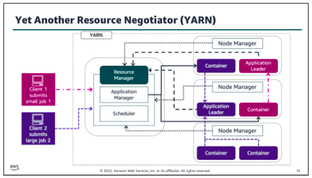
• Resource manager: Controls the use of resources within the Hadoop cluster, and manages the containers that are launched on each cluster node. The Resource Manager has two main components:
  • Scheduler: Allocates resources to the running applications, based on the resource requirements of those applications
  • Application manager: Accepts job submissions, negotiates the first container to run the Application Leader, and provides the service to restart the Application Leader on failure
• Node manager: Controls the use of resources within a single Hadoop cluster node, and monitors the containers that are launched on that cluster node.
• Application leader: Works with the Resource manager and Node manager to acquire cluster resource for processing tasks, before running and monitoring those tasks.
• Containers: Collection of cluster resources, such as memory and computer, that are allocated from a single cluster node to perform assigned processing activities.

Hadoop MapReduce:

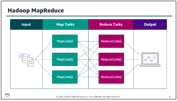
MapReduce is a framework for processing large datasets with a parallel, distributed algorithm on a cluster. Hadoop MapReduce simplifies writing parallel distributed applications by handling all of the logic, while you provide the Map and Reduce functions. The Map function maps data to sets of key value pairs called intermediate results. The Reduce function combines the intermediate results, applies additional algorithms, and produces the final output.

Multiple frameworks are available for MapReduce, such as Hive, which automatically generates Map and Reduce programs. The MapReduce framework is at the core of Hadoop and provides massive scalability across enormous numbers of Hadoop clusters. The framework is designed for fault tolerance, with each worker node periodically reporting its status to a leader node. The leader node can redistribute work from a cluster that doesn’t respond positively.

When running a big data job, the process begins as MapReduce splits the job into discrete tasks so that the tasks can run in parallel. Next, the mapper phase maps data to key value pairs (for example, the number of occurrences of each word on a data block). As soon as the mapper phase is finished, the next step is to shuffle and sort the data. During this step, for example, similar words are shuffled, sorted, and grouped together. The reduce phase counts the number of occurrences of words in the different groups and generates the output file.

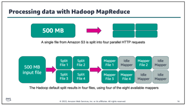
If you use HDFS to store your data, Hadoop automatically splits your data when it is stored in the HDFS cluster nodes. However, if you use Amazon Simple Storage Service (Amazon S3) to store your data, Hadoop splits the data by reading your files in multiple HTTP range requests whenever a processing job is started. The split size that Hadoop uses to read data from Amazon S3 varies depending on the Amazon EMR version that is being used. (Newer versions have larger split sizes.) The split size is generally the size of an HDFS block when operating on data that is stored in HDFS. Larger numbers provide less task granularity but also put less strain on the cluster NameNode.

In the example above the default split size has been set to 134,217,728 bytes (128 MB). Eight mapper processes are available to process the data. Big data processing needs to maintain pace with the volume and velocity of data, so in this instance the 500 MB input file will be split into four smaller files. Each of those files will use an available mapper for processing in parallel.

Code and commands:

Command	Description
hdfs dfs -ls [path]	List the contents of a directory in HDFS.
hdfs dfs -mkdir [path]	Create a directory in HDFS.
hdfs dfs -copyFromLocal [localSrc] [dst]	Copy files from the local file system to HDFS.
hdfs dfs -copyToLocal [src] [localDst]	Copy files from HDFS to the local file system.
hdfs dfs -mv [src] [dst]	Move files or directories within HDFS.
hdfs dfs -rm [path]	Delete files or directories from HDFS.
hdfs dfs -cat [path]	Display the contents of a file in HDFS.
hdfs dfs -tail [-f] [path]	Display the last kilobyte of a file in HDFS.
hdfs dfs -put [localSrc] [dst]	Copy files from the local file system to HDFS.
hdfs dfs -get [src] [localDst]	Copy files from HDFS to the local file system.
hdfs dfs -chmod [mode] [path]	Change the permissions of a file or directory in HDFS.
hdfs dfs -chown [owner]:[group] [path]	Change the owner and group of a file or directory in HDFS.
hdfs dfs -du [-s] [path]	Display disk usage for a file or directory in HDFS.
hdfs dfs -setrep [-R] [replication] [path]	Set the replication factor for files in HDFS.

Common Hadoop frameworks to process big data:

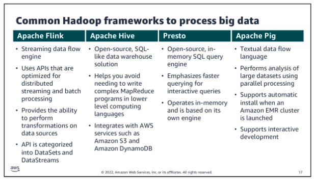
Hive to Presto

Before Presto, the data analysts at Facebook relied on Apache Hive for running SQL analytics on their multi-petabyte data warehouse. Hive was deemed too slow for Facebook’s scale and Presto was invented to fill the gap to run fast queries. In 2014, Netflix disclosed they used Presto on 10 PB of data stored in AWS S3. In 2016, Amazon announce a service called Athena that was based on Presto.

Apache Hive is a data warehouse software project, built on top of Apache Hadoop for providing data query and analysis. Hive gives an SQL-like interface to query data stored in various databases and file systems that integrate with Hadoop. Traditional SQL queries must be implemented in the MapReduce Java API to execute SQL applications and queries over distributed data. Hive provides the necessary SQL abstraction to integrate SQL-like queries (HiveQL) into the underlying Java without the need to implement queries in the low-level Java API. Since most data warehousing applications work with SQL-based querying languages, Hive aids the portability of SQl-based applications to Hadoop.

Features:

• Different storage types such as plain text, HBase, and others.
• Metadata stored in RDBMS, significantly reduces the time to perform semantic checks during query execution.
• Operating on compressed data stored in Hadoop ecosystem using algorithms including DEFLATE, snappy etc.
• Built-in user-defined functions to manipulate dates, strings, and other data-mining tools
• SQL-like queries (HiveQL), which are implicitly converted into Mapreduce, or Spark jobs.
• As any typical RDBMS, Hive supports all four properties of transactions (ACID)

By default, Hive stores metadata in an embedded Apache Derby database, and other client/server databases like MySQL can optionally be used.

Major components:

Metastore: stores metadata for each of the tables such as their schema and location, includes the partition metadata which helps the driver to track the progress of various data sets distributed over the cluster.

Driver: acts like a controller which receives the HiveQL statements, starts the execution of the statement by creating sessions and monitors the life cycle and progress of the execution.

Compiler: performs compilation of the HiveQL query, which converts the query to an execution plan.

Optimizer: performs various transformation on the execution plan to get an optimized DAG.

Executor: after compilation and optimization, the executor executes the tasks, interact with the job tracker of Hadoop to schedule tasks to be run.

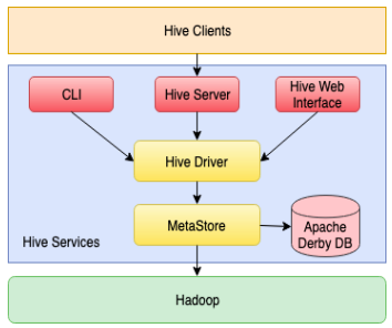
SELECT name
FROM employees
WHERE age < 30;

Pig

Apache Pig was originally developed at Yahoo Research for researchers to have an ad hoc way of creating and executing MapReduce jobs on very large data sets.

Apache Pig is a high-level platform for creating programs that run on Apache Hadoop. The language for this platform is called Pig Latin. Pig can execute its Hadoop jobs in MapReduce, Tez, or Spark. Pig Latins abstracts the programming from the Java MapReduce idiom into a notation which makes MapReduce programming high level, similar to that of SQL for RDBMS. Pig Latin can be extended using UDFs which the user can write in Java, Python, JS, and then call directly from the language.

Pig Latin is procedural and fits very naturally in the pipeline paradigm while SQL is instead declarative. In SQL users can specify that data from two tables must be joined, but not what join implementation to use. Pig Latin allows users to specify an implementation or aspects of an implementation to be used in executing a script in several ways. In effect, Pig Latin programming is similar to specifying a query execution plan, making it easier for programmers to explicitly control the flow of their data processing task.

SQL is oriented around queries that produce a single result. SQL handles trees naturally, but has no built in mechanism for splitting a data processing stream and applying different operators to each sub-stream. Pig script describes a DAG rather than a pipeline.

-- Load the employee records from the CSV file
employee_records = LOAD 'employee_records.csv' USING PigStorage(',') AS (name:chararray, age:int);

-- Filter employees younger than 30
young_employees = FILTER employee_records BY age < 30;

-- Select the names of young employees
young_names = FOREACH young_employees GENERATE name;

-- Store the names of young employees into an output file
STORE young_names INTO 'young_employees_output';

Oozie

(sounds like airflow for hadoop)

Apache Oozie is a server-based workflow scheduling system to manage Hadoop jobs. Workflows in Oozie are defined as a collection of control flow and action nodes in a DAG.

• Control nodes define the beginning and the end of a workflow (start, end, and failure nodes) as well as the mechanism to control the workflow execution path (decision, fork, and join nodes)
• Action nodes are the mechanism by which a workflow triggers the execution of a computation/processing task.

Oozie provides support for different types of actions including Hadoop MapReduce, Hadoop distributed file operations, Pig, SSH, and email. Oozie can also be extended to support additional types of actions.

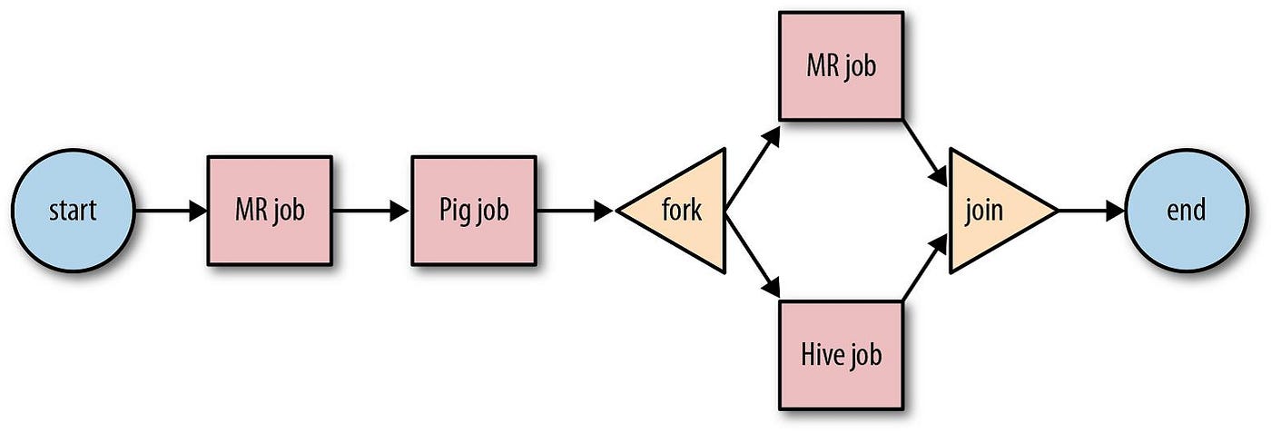
Apache Spark

Apache Spark is an open source, distributed processing framework that was created to address the limitations of MapReduce. Spark processes data in memory, reduces the number of steps in a job, and reuses data across multiple parallel operations. With Spark, only one step is needed, where data is read into memory, operations are performed, and the results are written back this results in a much faster processing. Spark is a cluster framework and programming model for processing big data workloads.

Spark also reuses data by using an in memory cache to speed up ML algorithms that repeatedly call a function on the same dataset. Data reuse is accomplished by creating DataFrames an abstraction over Resilient Distributed Dataset (RDD). DataFrames are a collection of objects that are cached in memory and reused in multiple Spark operations. This dramatically lowers the latency, which makes Spark multiple times faster than MapReduce especially for ML and interactive analytics.

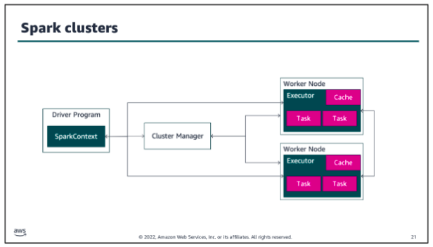
In Spark clusters, Spark applications run as independent sets of processes. The SparkContext object that resides within the driver program coordinates these processes. Spark connects to a cluster manager, which acquires executors from nodes within the cluster. These executors are responsible for running the computations and storing the data in cache for your application. The SparkContext object communicates directly with the executors, sending them tasks to be processed.

The components that make up the Spark framework are Spark Core, Spark SQL, Spark GraphX, Spark Streaming, and Spark MLlib. Let’s take a closer look at each of these.

As the name implies, Spark Core is the foundation of the platform. It’s responsible for memory management, fault recovery, scheduling, distributing and monitoring jobs, and interacting with storage systems. Spark Core is exposed through APIs built for Java, Scala, Python, and R. These APIs hide the complexity of distributed processing behind simple, high level operators.

Spark SQL is a distributed query engine that provides low latency, interactive queries up to 100 times faster than MapReduce. Spark SQL includes a cost based optimizer, columnar storage, and code generation for fast queries, while scaling to thousands of nodes.

Spark GraphX is a distributed graph processing framework that is built on top of Spark. GraphX provides ETL, exploratory analysis, and iterative graph computation to enable users to interactively build and transform a graph data structure at scale. It comes with a highly flexible API and a selection of distributed Graph algorithms.

Spark Streaming is a real time solution that uses Spark Core’s fast scheduling capability to do streaming analytics. Spark Streaming ingests data in mini batches and enables analytics on that data with the same application code that is written for batch analytics. This improves developer productivity because they can use the same code for batch processing and real time streaming applications.

Spark MLlib is a library of algorithms to do ML on data at scale. Data scientists can use R or Python to train ML models on any Hadoop data source, save them using MLlib, and import them into a Java or Scala based pipeline.

Ecosystem

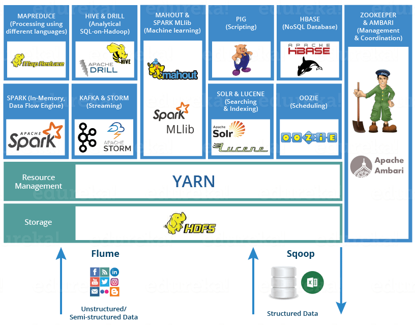
Amazon Cloud

Amazon EMR is a managed cluster platform. The service simplifies running big data frameworks, such as Apache Hadoop and Apache Spark, on AWS to process and analyze vast amounts of data. By using these frameworks and related open source projects, such as Apache Hive and Apache Pig, you can process data for analytics and business intelligence (BI) workloads. Additionally, you can use Amazon EMR to transform and move large volumes of data. You can move this data in and out of other AWS data stores and databases, such as Amazon S3 and Amazon DynamoDB.

With Amazon EMR, you have the ability to launch clusters in minutes, deploy multiple clusters, and resize clusters that are already running. By using these clusters, you can process your large volumes of data in a cost effective manner. Amazon EMR relies on HDFS and Amazon S3 for storage. Therefore, you can store input and output data in Amazon S3 while using HDFS to store your intermediate results. Finally, Amazon EMR provides the ability to perform automated installations of common big data projects such as Hive, Pig, and Spark, and run applications such as Hadoop, Spark, and Presto.

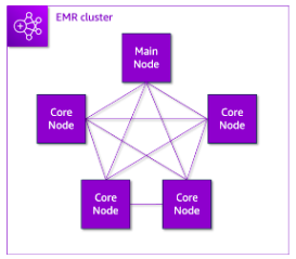
The central component of Amazon EMR is the cluster, which is a collection of Amazon Elastic Compute Cloud (Amazon EC2) instances. These EC2 instances are referred to as nodes, and each node has a role known as node type within the cluster. Each node type can have different software components, which further delineates its role in the cluster. Amazon EMR uses three node types: main, core, and task.

The main node is responsible for managing the cluster by running software components that coordinate data distribution and tasks to other nodes for processing. Every cluster has a main node, and you can create single node clusters that have only a main node.

Core nodes are responsible for running tasks and storing data in your cluster’s HDFS. Multi node clusters must have at least one core node.

Task nodes, which are optional, only run tasks. Task nodes don’t store data in HDFS, and you can add them at cluster launch or add them to an already running cluster to increase processing capacity. Additionally, you can terminate individual task nodes to reduce costs when they are no longer needed.