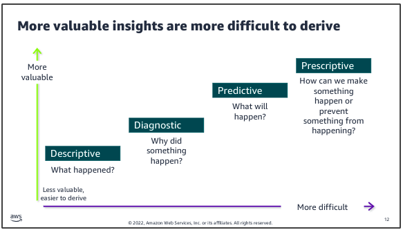
Data analytics:
- is the systematic analysis of large datasets (big data) to find patterns and trends to produce actionable insights
- uses programming logic to answer questions from data
- is good for structured data with a limited number of variables
AI/ML:
- is a set of fundamental models that are used to make predictions from data at a scale that is difficult or impossible for humans
- uses examples from large amounts of data to learn about the data and answer questions
- is good for unstructured data and where the variables are complex
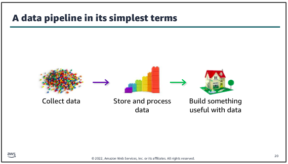
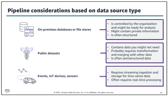
Data pipeline:
A data pipeline provides the infrastructure to turn data into insights and make data-driven decisions:
The number of variations and options to create a data pipeline are broad. The key to designing an effective decision making infrastructure is to start with the business problem to be solved or decision to be made. Then, build the pipeline that best suits that use case.
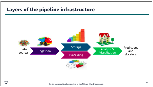
The infrastructure layers that you need to build include methods to ingest and store data from the data sources that you have identified. You need to make the stored data accessible for decision making processes. You must also create the infrastructure to process, analyze, and visualize data by using tools that are appropriate to the use case.
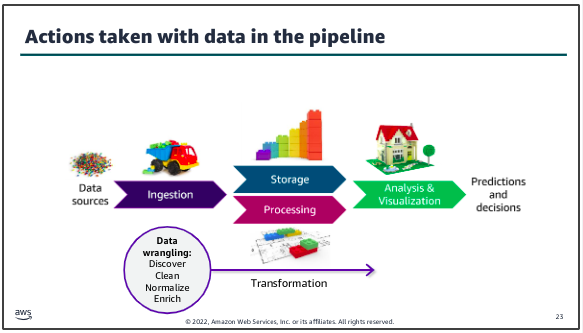
Data will almost always be transformed as it moves through the pipeline. This might include modifying the format to support a specific analysis tool or replacing values (for example, zeroes in place of nulls). You might also augment the dataset by filling in gaps or enriching it with additional information. For example, in traditional data science architectures, the extract, transform, and load (ETL) process takes data from one source, performs some type of transformation on it, and then loads it into another location where the analysis is done.
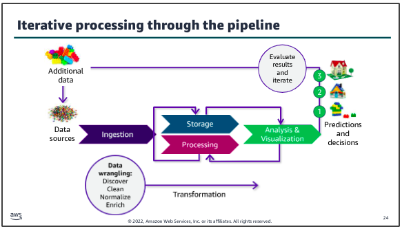
Another key characteristic of deriving insights by using your data pipeline is that the process will almost always be iterative. Here, after reviewing those results, they determined that additional data could improve the detail available in their result, so an additional data source was tapped and ingested through the pipeline to produce the desired result.
Example:
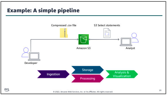
The dataset to be ingested into the pipeline is a .csv file that contains structured data. A developer uses a utility to compress the file, then uploads the file to an S3 bucket for storage. The data science team who will analyze the data can use S3 Select statements to directly query the data in Amazon S3.
To the AWS:
AWS Management Console: The starting point for interacting with AWS services is a web-based interface for accessing and managing AWS resources. It provides GUI that allows users to interact with various AWS services without needing to use the command line or write scripts. Once logged into the AWS Management Console, you’re presented with a list of AWS Services.
AWS Cloud9: A cloud-based IDE provided by AWS that allows you to write, run, and debug code with just a browser. It includes a code editor, debugger, and terminal. Cloud9 is particularly useful for developing serverless applications, allowing you to execute code in a cloud environment without needing to manage a local IDE setup. Each Cloud9 environment is essentially a virtual machine (VM) that AWS Cloud9 provisions and manages to provide an IDE in the cloud.
CloudFormation Template: AWS CloudFormation is a service provided by AWS that enables users to model and manage infrastructure resources in an automated and secure manner. The CF template is a text file that describes all the AWS resources you need to deploy to run your application. AWS CloudFormation provides a way to model and set up your AWS resources so that you can spend less time managing those resources and more time focusing on your applications that run in AWS. For example:
CloudFormation Stack: A stack implements and manages the group of resources that are outlined in your template. You can manage the state and dependencies of those resources together. Think of a CloudFormation template as a blueprint, and the stack is the actual instance of the template that creates the resources:
create_bucket.yml::
AWSTemplateFormatVersion: "2010-09-09"
Description: "TEST for S3 infrastructure"
Resources:
  S3Bucket:
    Type: 'AWS::S3::Bucket'
    Properties:
      BucketName: !Join
        - "-"
        - - "ade-my-bucket"
          - !Select
            - 0
            - !Split
              - "-"
              - !Select
                - 2
                - !Split
                  - "/"
                  - !Ref "AWS::StackId"
      PublicAccessBlockConfiguration:
        BlockPublicAcls: True
        BlockPublicPolicy: True
        IgnorePublicAcls: True
        RestrictPublicBuckets: True
      VersioningConfiguration:
        Status: Enabled
      BucketEncryption:
        ServerSideEncryptionConfiguration:
          - ServerSideEncryptionByDefault:
              SSEAlgorithm: 'aws:kms'
              KMSMasterKeyID: KMS-KEY-ARN
The CloudFormation templates does the following:
- Creates an S3 bucket
- Blocks public access to the bucket
- Enables versioning for the bucket.
- Enables server-side encryption for the bucket.
To validate the CloudFormation template, run the following command in terminal of Cloud9:
aws cloudformation validate-template --template-body
file://create_bucket.yml
Now you will create a CloudFormation stack from the template:
aws cloudformation create-stack --stack-name ade-my-bucket  --template-body
file://create_bucket.yml
To verify that the stack created the necessary resources, run the following command:
aws s3api list-buckets
To delete the stack, run the following command:
aws cloudformation delete-stack --stack-name ade-my-bucket
Datasets to S3:
To copy the dataset into the S3 bucket, run the following command:
aws s3 cp lab1.csv s3://<LAB-BUCKET-NAME>
To confirm that the file was added to the bucket:
aws s3 ls s3://<LAB-BUCKET-NAME>
Quering:
Amazon S3 is an object storage service that offers industry-leading scalability, data availability, security, and performance. When we talk about Buckets in AWS, we’re typically referring to storage contains in S3 where data is organized. Amazon S3 Select feature allows to retrieve only a subset of data from an object in S3 by using simple SQL expressions.
Security and storage:
The base level of encryption for all Amazon S3 buckets is server-side encryption with S3 managed keys (SSE-S3), ensuring that every object is encrypted. Users can modify the storage class of an object stored in Amazon S3 via the AWS Management Console. Amazon S3 offers several storage classes designed to suit different use cases based on data access patterns, durability, availability, and cost.
Compression:
Amazon S3 offers several storage classes designed to suit different use cases based on data access patterns, durability, availability, and cost. Amazon S3 offers several storage classes designed to suit different use cases based on data access patterns, durability, availability, and cost.\
zip lab lab1.csv

gzip -v lab1.csv

ls -la
To upload the GZIP version of the dataset to the S3 bucket, run the following commands:
aws s3 cp lab1.csv.gz s3://<LAB-BUCKET-NAME> --cache-control max-age=60
Managing and testing restricted access for a team member:
When the data science team uses the workflow that you have created, team members should only be allowed to access certain AWS services and features, such as S3 Select to query datasets. When the data science team uses the workflow that you have created, team members should only be allowed to access certain AWS services and features, such as S3 Select to query datasets. In this task, you will review the data science team’s IAM group and associated IAM policy. You will act as Paulo to test a few actions to determine whether the group and policy have permissions to access the dataset in Amazon S3.
IAM: An IAM in AWS is a collection of IAM users. It allows you to specify permissions for multiple users, which can make it easier to manage permission for those users as a group. Instead of assigning permissions to each user individually, you can assign them to a group, and all users in that group automatically inherit those permissions. It exists as a service within AWS.
Note: Federated users are authenticated through an external identity provider, and AWS IAM roles are assumed based on the federation policy. To test whether a user can perform certain AWS CLI commands, you can pass the user’s credentials as back variables (AK and SAK) with the command.
AWS_ACCESS_KEY_ID=$AK AWS_SECRET_ACCESS_KEY=$SAK ...
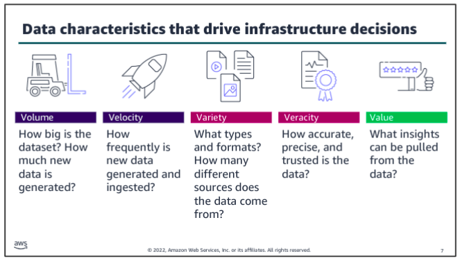
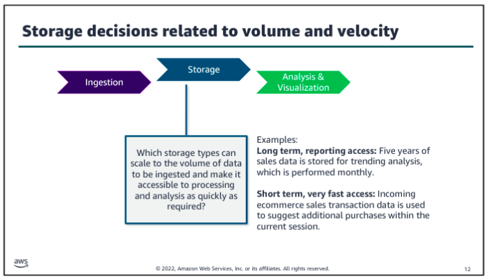
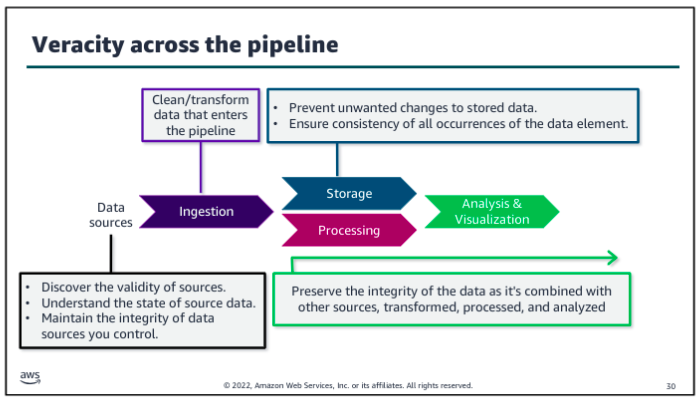
Elements of Data: Five V’s
The five Vs are volume, velocity, variety, veracity and value.
Consider volume and velocity together because you will make infrastructure decisions about how to collect, store, and process data based on the combination of how much data you need to ingest and how quickly you will ingest it.
Variety and veracity both relate to the data itself - what type of data is it and what’s the quality of it. Data engineers and data scientists will transform and organize the data based on its variety and veracity to make it useful for analysis.
Value is about ensuring that you are getting the most out of the data that you have collected. Value is also about ensuring that there is business value in the outputs from all that collecting, storing, and processing.
How Vs affect data pipeline?
Data Pipeline Patterns:
With the rise of the internet, the three tier architecture became prominent. Applications were split into groups by function: a presentation tier served as the user interface, an application tier handled the business logic and processing, and a data tier provided long term, persistent storage. Again this increased the scalability of applications because each tier could be scaled independently.
The most recent architectural trend, which aligns well to cloud best practices, is to move to microservices. With microservices, you split your application into different services based on functionality. For example, rather than having one application that handles both your inventory data and order history data, you might split those into two separate services that are focused on their domain. This split allows the two services to scale independently and provides more agility between development teams.
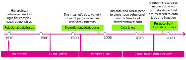
In the 1980s, data warehouses evolved as a way to separate operational reporting, which requires read-heavy quering across a full dataset, from the applications’ transactional database, which is focused on fast reads and writes in a much smaller set of records. OLAP database are optimized for reporting whereas OLTP databases are designed for transactions, such as creating an order or making an ATM withdrawl. The ETL process was introduced to extract data from OLTP databases, transform it, and then load into the data warehouse.
Administrators could scale vertically - that is, increase the size and speed of the database - but there wasn’t an easy way to scale horizontally - that is, to distribute the load across multiple database. Big data systems or frameworks addressed this shortcoming in the 2000s.
Work was still mostly done by batching at some scheduled interval. Batch processing created a lag between the arrival of new data and its being included in analytics results. The continually increasing volume and velocity of new data meant that the time between batches created an increasingly large gap in the timeliness of data being processed. To find a balance between value and complexity, Nathan Marz proposed the lambda architecture an approach which combines the use of batch processing with stream processing to support close to real time insights.
Modern AWS:
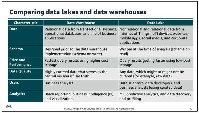
The goal of the modern data architecture is to store data in a centralized location and make it available to all customers to perform analytics and run AI/ML applications. But that does not mean that you have one data store - only that you have a single source of truth. A data lake provides the centralized repository of data and is integrated with the other types of data stores and data processing systems that were described in the previous section. Data might be queried directly from the lake, or it might be moved to and from other purpose built tools for processing.
The movement of data among the lake and other integrated services falls into three general types: outside in, inside out, and around the perimeter.
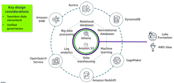
Amazon S3 provides storage for structured and unstructured data and is the storage service of choice to build a data lake on AWS. With Amazon S3, you can cost-effectively build and scale a data lake of any size in secure environment with high durability. With Amazon S3, you can also use native AWS services to run big data analytics and AI/ML applications. Amazon Athena is shown directly on the data lake to illustrate that it provides interactive querying of data directly in Amazon S3.
Two additional service provide movement and governance for this architecture. AWS Glue facilitates data movement and transformation between data stores, which helps to prepare data for analytics and ML much more quickly than traditional ETL methods. AWS Lake Formation was built to make it easier to manage time consuming tasks that are related to loading, monitoring, and managing data lakes. Lake Formation helps to catalog data and classify and secure it for different types of access.
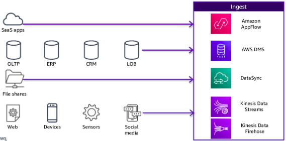
Ingestion Pipeline:
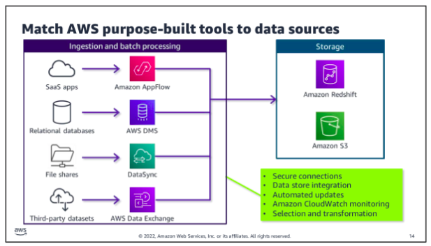
In the ingestion layer, you can match AWS services to source data types so that you can more easily bring in different types of data. Most services also integrate directly with storage layer components. The storage layer has two sub-layers. One provides storage, and the other provides the catalog that holds the metadata about the databases that are being stored.
The ingestion layer uses individual purpose-built AWS services to match the unique connectivity, data format, data structure, and data velocity requirements of source types and to deliver them to the storage layer components:
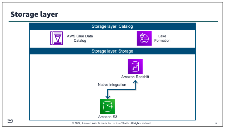
Storage Pipeline:
Data is ingested into the storage layer.
The data storage layer is responsible for providing durable, scalable, and cost effective components to store and manage vast quantities of data. In the AWS architecture, Amazon Redshift and Amazon S3 provide unified, natively integrated storage. The catalog layer in the storage layer is responsible for storing business and technical metadata about datasets that are hosted in the storage layer. This metadata supports the ability to find and query data that is stored in the data lake and the data warehouse. In the AWS architecture, Lake Formation and AWS Glue work together to collect and store metadata and make it available when needed. The catalog makes it easier for consumers to search for and explore the available data.
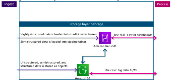
The native integration between Amazon S3 and Amazon Redshift means that you can ingest data as is into Amazon S3 and then prepare it for the data warehouse as needed. This lets you offload historical data from warehouse storage into a more cost-efficient storage tier in Amazon S3, which reduces the cost of storage.
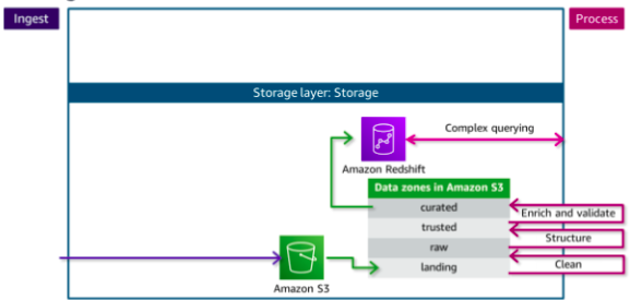
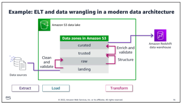
Each zone represents a different state of data and is represented by a bucket or prefix in Amazon S3. Zones include landing, raw, trusted, and curated. Data might pass through each zone as it is cleansed, normalized, augmented, or transformed in some other way. Transformed data is saved into a zone that matches its readiness to be consumed.
Data being ingested into the Amazon S3 data lake arrives at the landing zone, where it is first cleaned and stored into the raw zone for permanent storage. Because data that is destined for the data warehouse needs to be highly trusted and conformed to a schema,the data needs to be processed further.
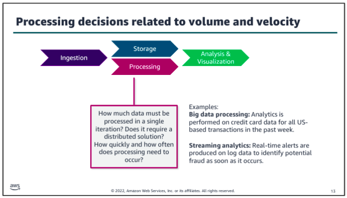
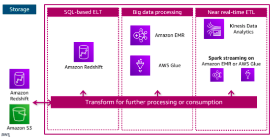
Processing Pipeline:
The components in the data processing layer are responsible for transforming data into a consumable state. The processing layer provides purpose built components that enable a variety of data types, velocities, and transformations. Each component can read and write data to both Amazon S3 and Amazon Redshift in the storage layer, and all can scale to very high data volumes. Each pipeline reads data from the storage layer, processes it using temporary storage as needed, and then writes it to the appropriate location in the storage layer.
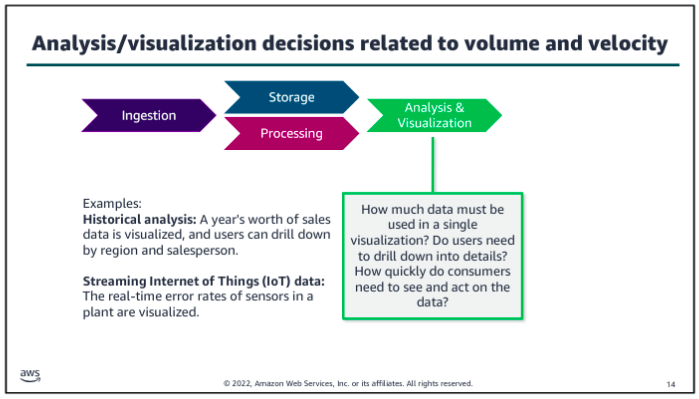
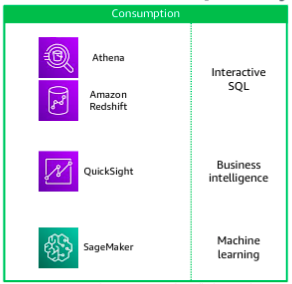
Consumption Pipeline:
The data consumption layer is responsible for providing scalable and performant components that use unified interfaces to access all the data and metadata in the storage layer. The consumption layer democratizes access to datasets for different types of users across the organization and enables different analysis methods. Each method has access to combine data from the data warehouse, which is stored in traditional schemas, and data in the lake, which is stored in open formats.
To the AWS:
However, she can’t use S3 Select with multiple files. Therefore, she would like the ability to query multiple files in the same S3 bucket and aggregate the data from these files into the same database. She also wants to be able to transform the dataset metadata, such as column names and data type declarations. This information is part of the dataset’s schema when the data is stored as a relational database.
Athena is an interactive query service that you can use to query data that is stored in Amazon S3. Athena stores data about the data sources that you query. You can store your queries for reuse, and you can share them with other users.
Query editor:
You created an AWS Glue database and table by using Athena query editor. You connected an S3 dataset to the table and defined the schema for the table using the bulk add columns feature. After you created the table, you learned how to preview the data by using the preview table feature. An external table stores only the metadata Hive (like the table schema) but the data itself is stored outside, such as, Amazon S3. The statements typically are part of Hive script or executed in an environment that can run HiveQL, such as AWS Athena.
Query optimization through query:
Three possible strategies that you can use to minimize your costs and improve performance are compressing data, bucketizing data, and partitioning data.
Compressing data: Compress your data by using one of the open standards for file compression (such as Gzip or tar). Compression results in a smaller size for the dataset when it’s stored in Amazon S3. The cardinality of your data also affects how you should optimize your queries. There are two options to optimize based upon high or low cardinality. These are:
Bucketizing data: For high cardinality with data, store records in distinct buckets (not to be confused with S3 buckets) based upon a shared value in a specific field. Considering bucketizing data as part of the preprocessing phase of your data pipeline. For example, data for a single month can be bucketized separately from the original dataset, which contains data for an entire year.
Partitioning data: You can also use partitions to improve performance and reduce cost Partitioning is used with low-cardinality data, which means that fields have few unique or distinct values. For example, paytype (cash, credit, unknown) is an excellent column to use to create partitions.
Athena views:
Athena supports only one SQL statement at a time, but you can use views to combine data from various tables. You can also use views to optimize performance by experimenting with different ways to retrieve data and then saving the best query as a view.
Athena CloudFormation:
The team wants to share the queries with other departments, but they use other accounts in AWS. The best solution is to build a CloudFormation template for each query. The template can be shared with other departments and deployed as needed.
Example:
AWSTemplateFormatVersion: 2010-09-09
Resources:
  AthenaNamedQuery:
    Type: AWS::Athena::NamedQuery
    Properties:
      Database: "taxidata"
      Description: "A query that selects all fares over $100.00 (US)"
      Name: "FaresOver100DollarsUS"
      QueryString: >
                    SELECT distance, paytype, fare, tip, tolls, surcharge, total
                    FROM yellow
                    WHERE total >= 100.0
                    ORDER BY total DESC
Outputs:
  AthenaNamedQuery:
    Value: !Ref AthenaNamedQuery
Ingestion ETL and ELT
The ingestion process incorporates extracting data from a source that isn’t already available in your pipeline, loading the data into some type of temporary storage in the pipeline, and processing the data by transforming it before or after the data is loaded into more permanent storage. The type and scope of transformations, and where they occur across the data pipeline, highly depend on the business need and the nature of the data that is being ingested.
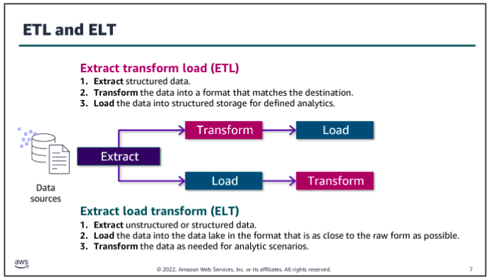
The trend towards collecting high volumes of unstructured and semis-structured data and the desire to make the data available for a variety of uses led to to a different approach for data ingestion: ELT. With an ELT approach, data is extracted from its source and transformed only enough to store it in a consumable but relatively raw state in a data lake. Transformations that might be needed for specific uses are done later, as customers access data and build analytics solutions with it.
Benefits of ETL:
ETL stores data that is ready to be analyzed, so it can save time for an analyst. If analysts routinely perform the same transformations on the data they analyze, it might be more efficient to incorporate those transformations into the ingestion process. So, with ETL, you trade longer transformation processing time before the data is available for faster access when you are ready to query it.
Another advantage of performing transformations up front is that you can filter out personally identifiable information (PII) or other sensitive data that could create a compliance risk. If you never store the sensitive data, you reduce the risk without the need to evaluate additional security measures.
Benefits of ELT:
With ELT, the process to get the raw data into your pipeline can be quicker because you aren’t required to transform the data as much before making it available in the data lake. So, with ELT, your trade-off is that you get the raw data available more quickly, but you spend more time to transform the data when you’re ready to work with it.
Another advantage of storing the raw data and only transforming it downstream is that changes to the transformation (for example, including additional fields or formatting data differently) would be run against all the historical data that was loaded when the transformation is updates. If the transformation occur before you load the data, your changes can apply to new data that is ingested, but it might be impossible or difficult to apply them to historical data.
Which to use?
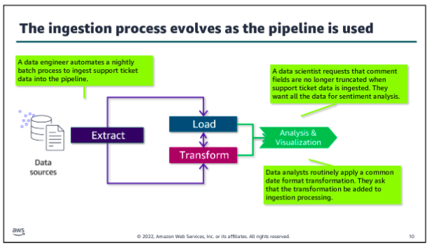
In modern architectures, ETL and ELT approaches are blurred. Each role that works with the pipeline might perform a different part of the ingestion and transformation process by using different tools and access. For example, the data engineer might use an ingestion tool that handles common cleaning or formatting transformations before loading a dataset into your data lake. Additional transformations might only occur only when the data is pulled for a particular analytics use case. The data analyst might apply a set of transformations on the ingested data to prepare it for a specific report. A data scientist might perform additional discovery and transformation on the ingested data to investigate hypotheses about relationships within the data.
As a patterns of use and understanding of the dataset evolve, you might revisit where and how transformations occur. For example, if many analysts perform the same recurring transformation to work with a dataset, adding those transformation into the processing that occurs before the data is loaded might improve performance or reduce costs.
Alternatively, you might recognize additional needs that you could serve by reducing the amount of transformation that is performed before loading the data. For example, you might truncate a large field to save costs, but a data scientists determines that there’s value in the truncated field and asks you to remove that transformation.
As the data engineer, you want to monitor how the pipeline performs, how it is accessed and used, and how you might modify your processes to optimize the value.
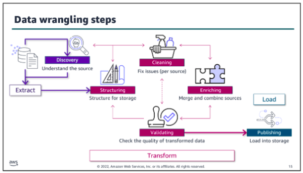
Ingestion wrangling
Regardless of when data is transformed, the data engineer needs to develop methods to extract and combine disparate data sources into a useful dataset. Data analysts and data scientists need to explore data, test hypotheses, and determine how to enrich or modify their dataset to meet their business needs. The term data wrangling reflects the complexity and messiness of transforming large amounts of unstructured data or sets of structured data with multiple schemas across multiple sources into a meaningful set of data that have value for downstream processes or users.
The overall ingestion and data wrangling process could be as simple as opening a source file in Microsoft Excel, manipulating columns and individual values in a spreadsheet, manually checking the validity of the data, and then saving it as a .csv file and uploading to Amazon S3 bucket. At the other end of the spectrum, complex transformations might be needed to support high volumes of incoming data for an ML application. The data engineer and data scientists might use a variety of scripts and tools to wrangle the data for this use case.
There is overlap between the ingestion, storage, and processing layer concepts. It’s important to remember that the defined layers help to describe the activities that are performed and tools that are used as data moves through and is transformed in the pipeline. But pipeline activities are iterative within and across layers.
Data discovery:
The data discovery step is iterative, and different roles might look for different things at this step. As a data engineer, you need to find sources that you think might be useful, query them, and analyze the raw data to decide whether the sources have value for your business purpose. Key tasks of this step include following:
- Decide if a source seems to serve your business purpose. If it does:
- Identify what relationships exist within and between raw data sources that you expect to use.
- Determine how you should organize the data to make it easy. For example, what fold structure is appropriate? What’s the best way to mange file size? How should you partition your target database table?
- Based on your analysis of the data relationships, formats and organizational requirements, determine what tools you need. Also, determine what you have available to store, secure, transform, and query the type of data in each source.
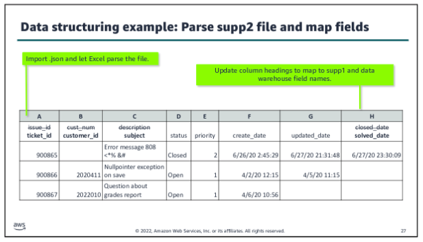
Data structuring:
The structuring step is the second defined step within the data wrangling process, following discovery. Data structuring is about mapping from the source file or files into a format that supports combining it with other data and storing it for its intended purpose. A key goal of this step is to optimize the structure of the raw dataset to minimize costs and maximize the performance of your processing pipeline. Key tasks:
- Organize storage.
- Parse the source file or files.
- Map fields.
- Manage file size.
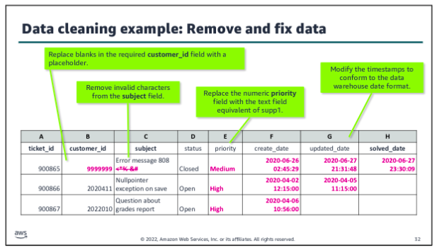
Data cleaning:
The cleaning step is the third defined step within the data wrangling process, following structuring. In the data cleaning step, you start to make the raw data ready for use in your pipeline. Usually, at this step, cleaning is per source, based on the characteristics of that source. Data cleaning includes tasks such as the following:
- Remove unwanted data.
- Fill in missing data values.
- Validate or modify data types.
- Fix outliers.
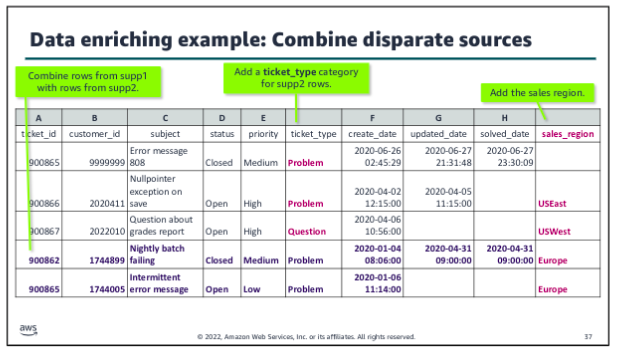
Data enriching:
The enriching step is the fourth defined step within the data wrangling process, following cleaning. In the data enriching step, you start to pull together related data from disparate sources to create the dataset that you need for your analysis. At this stage, you start to merge or combine data from different sources to support your use cases. Enriching might also include aggregations or other calculations that are added as new fields to the dataset.
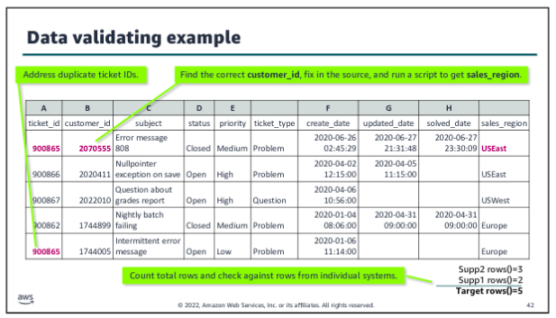
Data validating:
The validating step is the fifth defined step within the data wrangling process, following enriching. In the data validating step, you make sure that the dataset you have created for your analytics or ML use case has the veracity that you need. Validating has some similarities with the cleaning step. The initial cleaning step focuses on making sure that the data is suitable to successfully load into your pipeline. But the validating step is about ensuring the integrity of the dataset that you have created through the structuring, cleaning, and enriching steps for the combined source files.
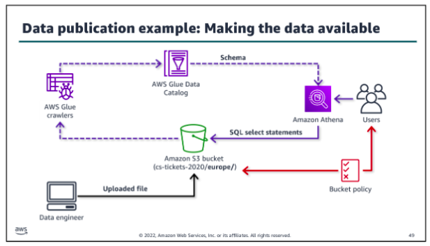
Data publishing:
The publishing step is the sixth defined step within the data wrangling process, following validating. In the data publishing step, you make the dataset available for use within the pipeline. During publishing, you apply your structuring decisions. You need to write data to the appropriate folders or partitions, and apply the file management techniques that you decided on. For example, you might split files to make them load faster and compress them to save on storage costs in the data lake:
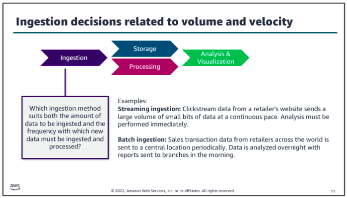
Ingestion by Batch or by Stream
To generalize the characteristics of batch processing, batch ingestion involves running batch jobs that query a source, move the resulting dataset or datasets to durable storage in the pipeline, and then perform whatever transformations are required for that use case. Batch processing might be started on demand, run on a schedule, or initiated by an event. Traditional ETL uses batch processing, but extract, load, and transform (ELT) processing might also be done by batch.
The advantage of batch processing is its ability to process a large set of transactions that are collected over a period of time and perform complex and long running processing on the dataset. Batch processing is typically less costly and easier to manage if there’s no urgency to perform the analysis.
By contrast, once a stream is active, streaming records arrive and are put onto the stream continuously. Consumers continuously read records off of the stream and process them on a sliding window of time, often making them available for real-time analytics immediately. The processed records might also be written to durable storage for downstream consumption. The big advantage of streaming ingestion is the opportunity to review results and take action immediately. Data is ready for analysis with very low latency. Also, the stream is designed to handle high volume, high velocity unstructured data.
Batch ingestion:
To meet a data request, consider the ETL tasks that you must perform:
- Connect to your data source and select the data to be ingested.
- Identify the source schema and define the target schema so that you can map the fields properly.
- Transfer the data securely into the pipeline. Make sure that you establish mechanisms to audit the ingestion process to ensure the veracity of the data in the pipeline.
- Perform transformations and load the processed data into durable storage, where it can be accessed. You might use a transform/load approach, where the majority of transformations occur prior to loading into the storage layer. Or, you might use the load/transform approach by performing minimal transformations before loading the raw data into your storage layer.
To perform the set of tasks, you would write scripts to perform the steps, rather than entering them at a command line each time. For example, you might write scripts to securely connect to the source, run queries to get the desired data, and transfer that data to some type of staging storage where the transformations could be done. You would also look for ways to script the manual steps that are needed to structure, clean, enrich, validate, and publish the dataset.
So now you have a set of scripts to get the data that you want, transfer it to temporary storage, wrangle it, and write it to your storage layer. The next step is to create batch jobs to automate running the set of ETL scripts that you have created. You might schedule the batch jobs to run on a scheduler or based on an event.
Orchestration:
The last piece to making your batch ingestion pipeline production ready is to create a workflow to orchestrate when each job runs. You also need to handle interdependencies between jobs and related actions and parameters. For example, you need to manage what happens if one job fails or if a resource isn’t available.
Orchestration is especially important when you move beyond the simple example to a more complex ingestion process. For example, what if you were now asked to collect and include customer comments from the tickets to feed an ML model as part of analyzing the relationship between customer support experiences and contract renewals? Now you need to collect and wrangle an additional subset of unstructured data, and you would need to label it and take other steps to use it in an ML application. A workflow helps to manage the complexities of this type of ingestion.
Choose a development framework that provides flexibility for developers and also lets nondevelopers to build and run jobs easily. Offering low-code or no-code options to write ETL jobs and serverless options to run those jobs reduces the operational overhead for the data engineer. Select tools that allow for the variety of data types, sources, and formats that you might need to process. Where possible, choose tools that are purpose built to ingest the data type that you are using.
Tools:
AWS Glue is a data integration service that helps you to automate and perform ETL tasks as a part of ingesting data into your pipeline. You can also use the service to facilitate transformation and movement between data stores. AWS Glue features include:
- Automatically generate schemas from semi-structured data by using crawlers.
- Catalog data and get a unified view with the Data Catalog.
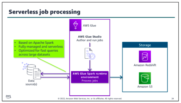
- Use AWS Glue Studio to author ETL jobs that bring data in from different sources and load it into a target
- Perform severless ETL processing in the AWS Glue Spark runtime engine.
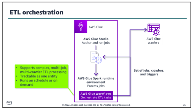
- Orchestrate complex ETL tasks with interdependencies by using workflows.
- Monitor, troubleshoot, and optimize ETL jobs and workflows.
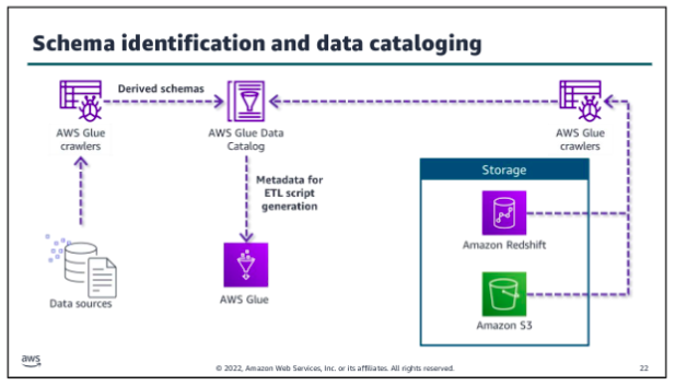
The AWS Glue Data Catalog stores metadata including schema information about data sources and targets of your ETL jobs. AWS Glue crawlers run on your data stores, derive schema from them, and populate the Data Catalog. Crawlers can run on many data stores, including Amazon S3, Amazon Redshift, most relational databases, and DynamoDB. By using the metadata in the Data Catalog, you can also automatically generate scripts with AWS Glue extensions. You can use these as your starting point to write your AWS Glue jobs.
Whether you use the scripts that the AWS Glue Data Catalog generates, you can use AWS Glue Studio, a feature of AWS Glue, to write your scripts and author jobs. You can also use the tool to run the jobs that you have created. You can run jobs on a schedule, on demand, or based on a specific event.
You can do the following with AWS Glue Studio:
- Pull data from an Amazon S3, Amazon Kinesis, or JDBC source.
- Configure a transformation that joins, samples, or transforms the data.
- Specify a target location for the transformed data.
- View the schema or a sample of the dataset at each point in the job.
- Run, monitor, and manage the jobs that were created in AWS Glue Studio.
When you run your AWS Glue job, the service extracts the data from the identified source or sources and performs the specified transformations in a runtime engine in a managed serverless environment. You configure some aspects of the runtime environment as part of setting up your jobs, but you don’t need to provision or manage servers. AWS Glue will also load the resulting dataset to the target storage location that you specify in your job.
The AWS Glue runtime engine is Apache Spark based. Spark is an open source, distributed processing system for big data. Spark is optimized to run fast queries across large datasets. AWS developed a performance optimized runtime for Spark for use with Amazon EMR. AWS Glue uses that same runtime engine.
Glue orchestration:
To orchestrate complex ETL processes, use AWS Glue workflows. Workflows work with the runtime engine to make it easier to design multi-job, multi-crawler ETL processes. You can run and track and track a workflow as a single entity. After you create a workflow and specify the jobs, crawlers, and triggers that are associated with it, you can run the workflow on demand or on a schedule:
Scaling considerations:
Batch goals are often about completing within a specific time frame, within a given budget, or with a certain threshold of accuracy. For example, your primary goal might be to make sure that daily batches are completed by a specific time to support a daily analysis task. Therefore, you would want to look at how long each step takes. Or you might be more focused on making sure that the resource usage of a job is within a specified budget, so you might focus on processing overnight over a longer period of time to reduce the cost of resources.
Of course, you want to look for steps that fail and determine if failures are related to scaling. For example, if a step times out while waiting for another step to complete or if a step fails because a resource is overwhelmed with requests, you might need to find ways to decouple those processes or scale individual resources up or out.
When you configure your batch jobs, it’s important to know how much data you are going to process, how often it’s updated, and how many different types of data you have. It’s also important to consider the type of transformations that need to occur on that data. For example, are you performing complex transformations that require a lot of data to be kept in memory at once, or are there quick individual transformations that happen per record?
Much of the tuning of the AWS Glue jobs will depend on how Spark distributes and processes your data based on the volume and type of data that is being ingested and the type of processing being performed on it. Spark is a distributed processing system, which means that is allocates processing across nodes. Spark takes steps to use its infrastructure to keep up with processing requests.

Glue AWS ETL:
As a data engineer, you might now always know the schema of the data that you need to analyze. AWS Glue is designed for this situation. You can direct AWS Glue to data that is stored on AWS, and the service will discover your data. AWS Glue will then store the associated metadata (for example, the table definition and schema) in the AWS Glue Data Catalog. You accomplish this by creating a crawler, which inspects the data source and infers a schema based on the data. You can direct the crawler to data that is stored in an S3 bucket, and the crawler discovers the data. Then, the crawler stores the associated metadata (the table definition and schema) in a Data Catalog. The team can now use crawlers to inspect data sources quickly and reduce the manual steps to create database schemas from data sources in Amazon S3. You can use Athena to query in a database that an AWS Glue crawler created. You ca also integrate an AWS Glue into a CloudFormation template.
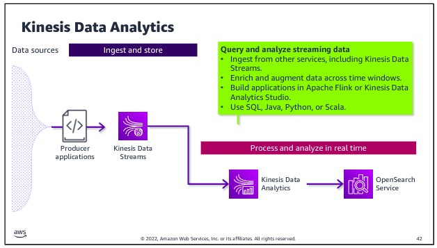
Kinesis for stream processing:
Amazon Kinesis Data Streams is specifically designed to ingest, process, and store streaming data for analytics. There are two paths for streaming ingestion. In the top path, streaming data is collected into the stream and stored for future use. In the second path, data is processed as it is ingested to feed real-time analytics. Producers put data onto a Kinesis Data Stream, which provides durable storage for the data. More than one producer can write to the stream. Consumers get the data from the stream and process it. The stream is a kind of buffer between the incoming data and the processors of that data. 0
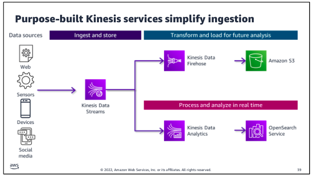
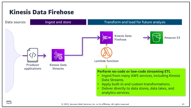
Kinesis Data Firehose is designed to ingest and deliver streaming data directly to data lakes on Amazon S3, as well as data stores and analytics services such as Amazon Redshift and Amazon OpenSearch Service. Kinesis Data Firehose also has the ability to run built-in transformations or custom transformations that you create by using a Lambda function that runs on the streaming data before it is delivered to specified destination.
Kinesis Data Analytics is purpose built to perform analytics on streaming data as it passes through the stream and to deliver data directly to tools for real-time analytics. For example, you might perform calculations to derive new fields or to aggregate values over a sliding time window within the incoming stream. You could then write the results to OpenSearch Service, where the results are available for Amazon OpenSearch Dashboards or other analytics and visualization tools.
Storage
Storage in the iterative data pipeline is far from a linear process. When data is ingested into the pipeline, it is placed in storage. The data can then be remove from storage, processed, and returned to storage for later use or to await additional processing and transformation.
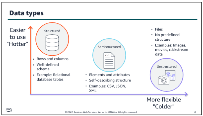
There are three types of cloud storage, each with their own advantages, disadvantages, and use cases. The three cloud storage types are block storage, file storage, and object storage.
The catalog layer in the storage layer stores business and technical metadata about datasets that are hosted in the storage layer. This metadata supports the ability to find and query data that is stored in the data lake and the data warehouse. In the AWS architecture, AWS Lake Formation and AWS Glue work together to collect and store metadata and make it available when needed. The catalog makes it easier for consumers to search for and explore the available data.
Amazon S3 provides you with object storage for structured and unstructured data. With S3 as the foundation of your data lake architecture, you can easily store, access, and query data from a multitude of data sources. You can then use this data immediately or place it in a low cost, long term storage solution, such as Amazon S3 Glacier, for later use and analysis.
Amazon Redshift uses SQL to analyze structured and semistructured data across data warehouses, operational databases, and data lakes. The service uses AWS designed hardware and ML to deliver the best price performance at any scale. Because the service is integrated with AWS services, including database and ML services, Amazon Redshift can help you handle complete analytics workflows.
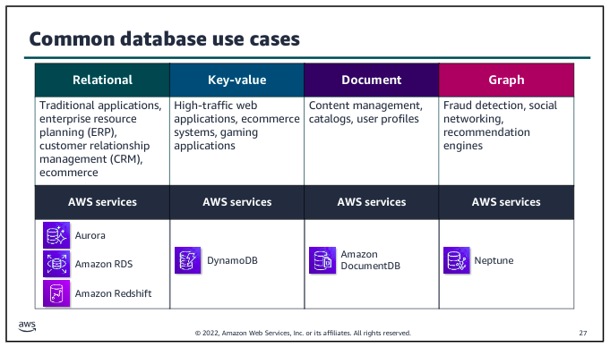
Purpose built databases:
Choosing the right purpose built database is key when selecting the application architecture that will support your analytics or ML workload. The database service that you choose will affect the volume and variety of what your application can handle, and determine what type of data is stored and the format it’s stored in.
Redshift Lab:
Clusters are the main infrastructure component of an Amazon Redshift data warehouse. A cluster is made up of one or more compute nodes. If a cluster has more than one node, then one of the nodes is the leader node, and the other nodes are compute nodes. Client applications interact with the leader node.
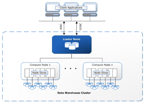
Amazon Redshift is deployed in a three-tier architecture. The cluster is placed within a private subnet of your VPC with web application servers in the public subnet. Users access the web application through a NAT gateway. The Redshift cluster is not available to the public internet, but port 5439 is configured within the security group to allow the application servers to access the Redshift database. You could add a bastion host to the public subnet to manage the cluster through SSH.
Amazon Redshift is deployed in a three-tier architecture. The cluster is placed within a private subnet of your VPC with web application servers in the public subnet. Users access the web application through a NAT gateway. The Redshift cluster is not available to the public internet, but port 5439 is configured within the security group to allow the application servers to access the Redshift database. You could add a bastion host to the public subnet to manage the cluster through SSH.
In Amazon Redshift, loading data from an Amazon S3 bucket into tables within a database involves using the COPY command. This command efficiently transfers data from S3 into Redshift tables, leveraging IAM roles for secure access permissions.
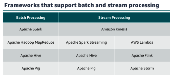
Big Data Processing
When you launch your cluster, you choose the frameworks and applications to install that best fit your data processing needs. Frameworks are the data processing engines that are used to process and analyze your data. You can select frameworks based on whether your data processing is batch, interactive, in-memory, streaming, or something else. Hadoop and Spark are the two most common frameworks that amazon EMR uses.
(shits too complicated for now)
Hadoop
=(this is from AWS course, check it AWS Data Pipeline Course)=
Apache Hadoop:
Hadoop is an open source framework that uses a distributed processing architecture. Hadoop maps tasks to a cluster of commodity servers for processing. Hadoop consists of four main components:
- Hadoop Distributed File System (HDFS);
- Yet Another Resource Negotiator (YARN);
- MapReduce; and
- Hadoop Common. Hadoop clusters consist of main nodes and worker nodes. In this format, main nodes are responsible for orchestrating jobs, while worker nodes are responsible for processing those jobs.
Benefits:
With Hadoop, you can store as much data as you like. You aren’t required to preprocess data prior to storing it; therefore, the framework provides increased flexibility. Hadoop also has a high degree of fault tolerance, thanks to node failover. If a node fails within a cluster, its tasks are redistributed throughout the other nodes within the cluster. Data loss is likewise prevented by having multiple copies of the same data stored throughout the cluster.
The Hadoop infrastructure is scalable as data processing and computing requirements grow, you can easily add nodes to support that growth in volume and velocity. Because it is an open source framework, Hadoop is free and capable of running on inexpensive hardware. Finally, you can use Hadoop to process structured, unstructured, and semistructured data. You can transform the data into a variety of other formats to integrate with your existing datasets, and you can store the data with or without a schema.
Challenges:
The framework does have a few challenges. Because of its open source nature, stability issues can arise as the framework is updated. You can avoid this challenge by running only the latest stable version. Hadoop also makes heavy use of the Java programming language a commonly targeted language that can leave the framework open to vulnerabilities. Lastly, security concerns are inherent to Hadoop. Lack of authentication and encryption can lead to questions about the veracity of the data.
Hadoop Distributed File System:
The Hadoop Distributed File System, or HDFS, is the distributed file system of the Hadoop framework. You can use HDFS to store huge amounts of data for further processing. HDFS and the Hadoop cluster use a hierarchical node architecture, which consists of a single NameNode that manages multiple DataNodes across clusters.
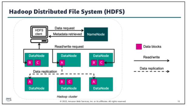
HDFS is typically used by applications that have large datasets, so it’s designed to provide high aggregate data bandwidth. To support data velocity while storing data, HDFS splits the data into small blocks - called data blocks - and stores those blocks across several nodes of the cluster. In the example, a large data file has been split into three data blocks.
Each block resides in a different data node when possible. To avoid losing data if a cluster node fails, HDFS replicates each block several times across different nodes. This enables a high degree of fault tolerance within HDFS. The number of times that a block is replicated is called the replication factor, and it’s a configurable setting. The cluster’s NameNode catalogs the metadata about each file that is stored in the cluster. The cluster DataNodes store the data blocks for each file that has been saved to HDFS.
Yet Another Resource Negotiator (YARN)
Yet Another Resource Negotiator also called YARN is a large scale, distributed operating system that is used with Hadoop. YARN makes the data that is stored in HDFS accessible for different processing. YARN dynamically coordinates the use of available Hadoop resources to schedule and perform that processing.
YARN has a few primary components:
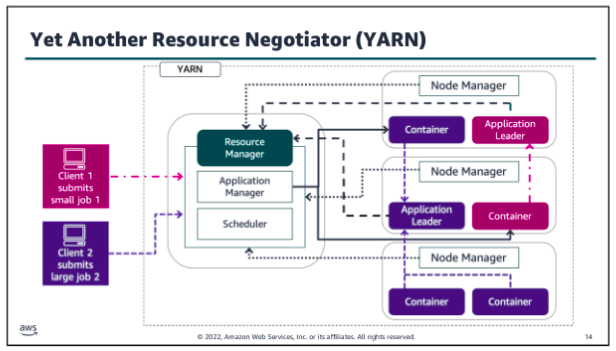
- Resource manager: Controls the use of resources within the Hadoop cluster, and manages the containers that are launched on each cluster node. The Resource Manager has two main components:
- Scheduler: Allocates resources to the running applications, based on the resource requirements of those applications
- Application manager: Accepts job submissions, negotiates the first container to run the Application Leader, and provides the service to restart the Application Leader on failure
- Node manager: Controls the use of resources within a single Hadoop cluster node, and monitors the containers that are launched on that cluster node.
- Application leader: Works with the Resource manager and Node manager to acquire cluster resource for processing tasks, before running and monitoring those tasks.
- Containers: Collection of cluster resources, such as memory and computer, that are allocated from a single cluster node to perform assigned processing activities.
Hadoop MapReduce:
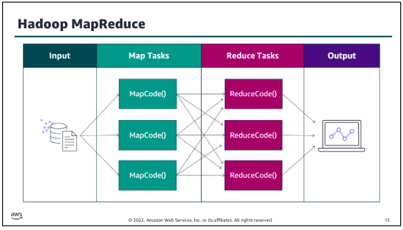
MapReduce is a framework for processing large datasets with a parallel, distributed algorithm on a cluster. Hadoop MapReduce simplifies writing parallel distributed applications by handling all of the logic, while you provide the Map and Reduce functions. The Map function maps data to sets of key value pairs called intermediate results. The Reduce function combines the intermediate results, applies additional algorithms, and produces the final output. Multiple frameworks are available for MapReduce, such as Hive, which automatically generates Map and Reduce programs. The MapReduce framework is at the core of Hadoop and provides massive scalability across enormous numbers of Hadoop clusters. The framework is designed for fault tolerance, with each worker node periodically reporting its status to a leader node. The leader node can redistribute work from a cluster that doesn’t respond positively.
When running a big data job, the process begins as MapReduce splits the job into discrete tasks so that the tasks can run in parallel. Next, the mapper phase maps data to key value pairs (for example, the number of occurrences of each word on a data block). As soon as the mapper phase is finished, the next step is to shuffle and sort the data. During this step, for example, similar words are shuffled, sorted, and grouped together. The reduce phase counts the number of occurrences of words in the different groups and generates the output file.
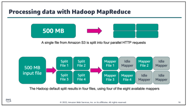
If you use HDFS to store your data, Hadoop automatically splits your data when it is stored in the HDFS cluster nodes. However, if you use Amazon Simple Storage Service (Amazon S3) to store your data, Hadoop splits the data by reading your files in multiple HTTP range requests whenever a processing job is started. The split size that Hadoop uses to read data from Amazon S3 varies depending on the Amazon EMR version that is being used. (Newer versions have larger split sizes.) The split size is generally the size of an HDFS block when operating on data that is stored in HDFS. Larger numbers provide less task granularity but also put less strain on the cluster NameNode.
In the example above the default split size has been set to 134,217,728 bytes (128 MB). Eight mapper processes are available to process the data. Big data processing needs to maintain pace with the volume and velocity of data, so in this instance the 500 MB input file will be split into four smaller files. Each of those files will use an available mapper for processing in parallel.
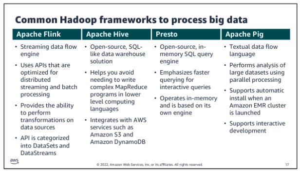
Common Hadoop frameworks to process big data:
Apache Spark
Apache Spark is an open source, distributed processing framework that was created to address the limitations of MapReduce. Spark processes data in memory, reduces the number of steps in a job, and reuses data across multiple parallel operations. With Spark, only one step is needed, where data is read into memory, operations are performed, and the results are written back this results in a much faster processing. Spark is a cluster framework and programming model for processing big data workloads.
Spark also reuses data by using an in memory cache to speed up ML algorithms that repeatedly call a function on the same dataset. Data reuse is accomplished by creating DataFrames an abstraction over Resilient Distributed Dataset (RDD). DataFrames are a collection of objects that are cached in memory and reused in multiple Spark operations. This dramatically lowers the latency, which makes Spark multiple times faster than MapReduce especially for ML and interactive analytics.
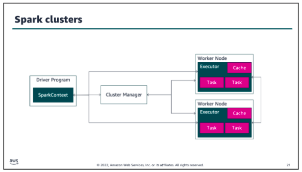
In Spark clusters, Spark applications run as independent sets of processes. The SparkContext object that resides within the driver program coordinates these processes. Spark connects to a cluster manager, which acquires executors from nodes within the cluster. These executors are responsible for running the computations and storing the data in cache for your application. The SparkContext object communicates directly with the executors, sending them tasks to be processed.
The components that make up the Spark framework are Spark Core, Spark SQL, Spark GraphX, Spark Streaming, and Spark MLlib. Let’s take a closer look at each of these.
As the name implies, Spark Core is the foundation of the platform. It’s responsible for memory management, fault recovery, scheduling, distributing and monitoring jobs, and interacting with storage systems. Spark Core is exposed through APIs built for Java, Scala, Python, and R. These APIs hide the complexity of distributed processing behind simple, high level operators.
Spark SQL is a distributed query engine that provides low latency, interactive queries up to 100 times faster than MapReduce. Spark SQL includes a cost based optimizer, columnar storage, and code generation for fast queries, while scaling to thousands of nodes.
Spark GraphX is a distributed graph processing framework that is built on top of Spark. GraphX provides ETL, exploratory analysis, and iterative graph computation to enable users to interactively build and transform a graph data structure at scale. It comes with a highly flexible API and a selection of distributed Graph algorithms.
Spark Streaming is a real time solution that uses Spark Core’s fast scheduling capability to do streaming analytics. Spark Streaming ingests data in mini batches and enables analytics on that data with the same application code that is written for batch analytics. This improves developer productivity because they can use the same code for batch processing and real time streaming applications.
Spark MLlib is a library of algorithms to do ML on data at scale. Data scientists can use R or Python to train ML models on any Hadoop data source, save them using MLlib, and import them into a Java or Scala based pipeline.
Apache HudI:
Apache Hudi is an open-source data management framework. Hudi is used to simplify incremental data processing and data pipeline development by providing record-level insert, update, upsert, and delete capabilities. Upsert refers to the ability to insert records into an existing dataset if they don’t already exist or to update them if they do. Hudi allows data to be ingested and updated in near real time by managing how data is organized in Amazon S3. Hudi maintains metadata of the actions that are performed on the dataset to help ensure that the actions are both atomic and consistent.