Database Management

A database management system is a collection of interrelated data and a set of programs to store and retrieve those data in a convenient and efficient.

Applications:

1. Enterprise information:
   • Sales: for customer, product and purchase information, payments, receipts, account balances, assets and other accounting
   • Human resources: for information about employees, salaries, taxes, benefits etc
2. Banking and finance:
   • Banking: for customer information, loans, accounts and transactions
   • Finance: holdings, stocks, bonds, real time market trading
3. Universities:
   • for students, courses, grades and human resources information
4. Airlines:
5. Telecommunication:
6. Web based services:
   • Social media
   • Online retailers
   • Online advertisers

Disadvantages of filesystems:

1. Data redundancy and inconsistency:

   • Same information may be duplicated in several files which leads to higher storage and access cost
   • Various files are likely to have different formats and programs may be written in different programming languages

2. Difficult in accessing data and isolation:

   • Need to ask system programmer to write the necessary application programs to retrieve data
   • As data are scattered across various files, writing new application programs is difficult

3. Atomicity problems:

   • The writes to system must happen in its entirety or not at all, which is difficult of ensure in conventional file systems

4. Concurrent-access anomalies:

   • race conditions

5. Security and backup problems:

Data Abstraction: Need for efficiency led database system developers to use complex data structures to represent data in the database, since many database-system users are not computer trained, developers hide the complexity from users through several levels of data abstractions, to simplify users’ interactions with the system:

1. Physical level:

   • Lowest level of abstraction describes how the data are actually stored
   • Describes complex low level data structures in detail such as dynamic tree structured indexes such as B Trees
   • Developers

2. Logical level:

   • Next higher level of abstraction describes what data are stored in the database, and what relationships exist among those data
   • Describes what tables are created and what are the links among them
   • Database administrators

3. View level:

   • Computer users see a set of application programs that hide details of the data types
   • Several views of the database are defined, and a database user sees some or all of these views
   • Users just interact with GUI to enter details and are not aware of what and how data are stored

The physical schema is hidden beneath the logical schema and can usually be changed easily without affecting application programs. Application programs are said to exhibit physical data independence if they do not depend on the physical schema and thus need not be rewritten if the physical schema changes.

Database instance: Databases change over time as information is inserted and deleted, the collection of information stored in the database at a particular moment is called an instance of a database

Database Schema: Overall blueprint of the database which specifies what fields will be present and what would be their types.

Data Model: Underlying structure of a database which includes collection of conceptual tools for describing data, data relationships, data semantics and consistency constraints

Note: Data model is a high level design which decides what can be present in the schema

1. Entity-Relationships:
	-ER model uses a collection of basic objects, called entities, and relationships among these objects
	-An entity is a thing or object in the real word that is distinguishable from other objets

2. Relational:
	-Uses a collection of tables to represent both data and relationships among those data
	-Each table has multiple columns, and each column has a unique name

3. Semi-structured:
	-Permits the specificaiton of data where individual data items of the same type may have different set of attributes
	-JSON and XML are widely used semi-strucutre data representations
	
4. Object-based:
	-Standards exist to store objets in relational tables

Database Languages:

1, DDL: Set of definitions that specifies a database schema
		create table account
			(
			account-number char(10),
			balance integer
			)
	
2, DML: Enables user to access or manipulate data as organized by the appropriate data model:
		select instructor.name
		from instructor
		where instructor.dept_name = 'History';
		
	> Procedurrals:
		require a user to specify what data are needed and how to get them
	> Declaratives:
		require a user to specify what data are needed without specifying how to get those data
	(Portion of a DML that involves information retrieval of information is a query language)

Database design using ERM: -In mapping the meanings and interactions of real-world enterprises onto a conceptual schema

ENTITIES:
- Entity: a thing or object in the real world that is distinguishable from other objects
- Entity set: a set of entities of the same type that share the same properties or attributes

RELATIONSHIPS:
- Relationships: an association among entities (not-jus-two)
- Relationship set: a set of relationships of the same types
	
Note: If E1, E2, ... , En are entity sets, then a relationship set R is a subset of
	{(e1, e2, ..., en) | e1 \in E1, e2 \in E2, ..., en \in En}
	where, (e1, e2, ..., en) is a relationship.
Hence, the entity sets E1, E2, ..., En participate in a relationship set R.

ATTRIBUTES:
- An entity or a relationship is represented by a set of attributes, are descriptive properties possessed by each member of the set
- (set bata arrow lagera euta oval shape ma dekhauni)
- Specialisations:
	> Composite: name ko first_name, middle_name, last_name bhako jastai, oval bata feri aru oval nikalni
	> Multivalued: phone numbers, double golo banauni
	> Derive: age from birthdate, dashed golo banauni

EXTRA INFOS:
1, Keys:
	- Allows to identify a set of attributes that suffice to distinguish entities from each other in a entity set or relationships from each other in a relationship set
	- Types:
	-Superkey: one or more attributes that, taken collectively, allow us to identify uniquely an entity in the given set
	-Candidatekey: minimal superkeys for which no proper subset is a superkey (aka. primary key)
	-Primarykey: only one candidatekey is primarykey
(dashed garinxa)

2, Mapping cardinalities: expresses the number of entities to which another entity can be associated via a relationship set
	
Note: For a binary relationship set R between entity sets A and B, the entities must:
	- One to one: An entity A is associated with at most one entity in B, and an entity in B is associated with at most one entity in A
	- One to many:
	- Many to one:
	- Many to many:
	
(arrow le denote garxa, arrow bhako one, nabhako many)
	
3, Participation constraints: participation of an entity set E in a relationship set R is said to be total if every entity in E participates in at least one relationship in R

(comment: aba kura garda A, B entity sets participate in a realtionship sets where A is total and B is partial jasari kura garna milxa)
	
(total participation of an entity set in a relationship double arrow le dekhauni)


4, Weak entity sets:
	- A weak entity set is one whose existence is dependent on another entity set, called its identifying entity set; instead of associating a primary key with a weak entitty, we use the primary key of the identifying weak entity, along with extra attributes, called discriminator attributes to uniquely identify a weak entity
	- The identifying relationsip is many-to-one from the ewak entity set to identifying entity set, and participation of weak entity set is total

(double box on weak entity and relatinoships, with dashed on discriminator attributes)

UNIVERSITY WALA SEXY EXAMPLE GOES HERE …

DESIGN PRINCIPLES: -Binary vs n-ary relationships: > Always possible to replace a n-ary relationship set by a number of distinct binary relationship sets > For a relationship set R, relating sets A, B and C, introduce a new entity set E, and create three relationship sets: Ra, relation E and A Rb, relation E and B Rc, relating E and C where, if R had any attributes, are assigned to entity set E

-Common mistakes not to make in any cases:
	>Not to use primary key of an entity set as an attribute of another entity set, instead of using a relationship
	(student ko attribute dept_name hunu bhayena)
	>Not to designate primary key attributes of the related entity sets as attributes of the relationshps stes
	(advisor relationships ma student ko ID ra instructor ko ID attributes hunu bhayena)
	>Not to use a relationships with a single valued attribute in a siutation that requires a multivalued attribute
	(section ra student ko relatinoship ma assigment, marks attributes hunu bhayena because it allows for only one assignemtn and marks for a studnet section combination)
	
-Entity sets versus relationship sets?

-Entity sets versus attributes:
	> Employee entity set with phone no. as one of the attributes
	> Employee entity set and phone no. participating in an relationship set 
		Ans: Generality requirement

-Placement of relationship attributes:
	> Attributes of one-to-many relationship set can be repositioned to only the entity set on the many side of the relationship, while for one-to-one, either one of the sets.

Relational Database: -A relational database consists of a collection of tables, each of which is assigned a unique name -The term relation is used to refer to a table, the term attribute refers to a column of a table while the term is used to refer to a row -A table of n-attriubtes must be a subset of: D1 \times D2 \times … \times Dn (D for domains) -Represented by schema: <table_name schema > = (att1, att2, …, attn)

Schema from ERD:

1. Strong entity sets:
	-Strong entity set E with distinct attributes is a table with same attributes as column headers
	student(ID, name, tot_cred)
	
	-For complex attributes:
	>For composite, create multiple attributes (firstname, lastname)
	>For derived are not explicitly represented there could be function for calculating it
	>For a multivalued attribute M, create a relation schema R with an attribute A that correspods to M and attributes corresponding to the primary key of the entity set or relationship set of which M is an attribute
		-For multivalued phone number of isntructOr, we create a relation schema:
			instrutor_phone (ID(underlined), phone_number(underlined))
		-Also add the constraint that the attribute ID references instruction relation
		
2. Weak entity:
	> A be a weak entity set with attributes a1, .., am. B be the strong entity entity set on which A depends then schema attribute is given by the union of them
		-primary key will be combination of primary key of identifying set and discrimator of the weak set
		section (course_id, sec_id, semester, year) all underlined
		-Also foregin key constaint that ensures that for each tuple represneitng a weak entity, there is a corresponding tuple represeneting the corresponding strong entity
	
3. Relationship sets:
	> The schema attributes consist of union of primary keys of each entity participating in relationship and the attributes of the relation itslef
	> Relationship set R with distinct attributes is a table formed by union of the same attributes with primary keys of entity sets participating in R
	>Also we create foreign key constraints on the relation schema R as follows: FOr each entity set Ei realted by relationshps R we create a foregin key contraint from relationship schema R, with the attributes of R that were derived from the primary key attributs of E refereing the primary key of the relation schema representing Ei
	>Ex: advisor relationship:
		adivsor(s_ID underlined, i_ID underlined) from relationship between student and instrutor

4. Linking weak entity set to strong:
	> In general, The schema for the relationship set linking weak entity set to its corresponding strong entity set is redundant and does not need to be present in a relational database design based upon an ER diagram
			
5, Combination of tables:
		- A many-to-one relationship set AB from entity set A to entity set B results in three tables A, B and AB
		- On condition that participation of A on relationship is total then combine A and AB to form a single table consisting of union of columns of both tables
		-The primary key of the combined schema is the primary key of the entity set into whose schema the relationship set schema was merged.
		
		-In the case of one to one relationshps, the relation schema for the relationship can be combined with the shemas for either of the entity sets

		-Drop the constraint referencing the entity set into whose schema the relationship set schema is merged, and add the other foreign key constraint to the combined schema

Extended ER featurs: -Generalization: tei OOP ko idea: can be total or partial denoted by a triangel -Aggregation: some ERD ko part nai box bhitra rakhera considered a high level entity for example (employee does job on branch ternary relationship ho) yeslai euta box ma rakhni ani teslai euta entity maanera manages by manager garni

FROM YOUTUBE:

1. Mapping of regular entity types: -For each regular strong entity type E in the ER schmea, create a relation R that incldues all the simple attributes E -(composite attributes xa bhane tesko indiviual lai lekheko xa) -Choose one of the key attributes of E as the primary key for R. If chosen key E is composite, the set of simple attributes that form it together will form the primary key of R

2. Mapping of weak entity types: -For each weak entity type W in the ER schema with owner enitty E, create a relation R and inclue all simple attribute (or simple part of compostie) of W as attributes of R -In addition, include as foreign key attriubtes of the primary key attributes of the relatinos that correspond to the owener entity types -The primary key of R is the combinarion of the primary key(s) of th owner(s) and the partial key of the weak entity type W, if any -(tyo duita bich ko relationship lai kei chaidain rey)

3. Mapping of 1:1 relation types -Three approach: >Foreign key apporach: Choose one of the relation S and include a foreign key in S the primary key of T. It is better to choose an entity type with total participation in R in the role of S (Means that total partiipation wala table ma arko table ko primary key lai foreign key banayera rakhni)

    >Merge relation option: An alternate mapping of a 1:1 relationship type is possible by mering the two entity types and the relationship into a single realtino. This may be appropriate when both particpation are total
    (attributes lai merge gardini ani duita ko madhye jaslai primary key banaye ni hunxa)
   
    >Cross refernce or relationship relation: Set up a third relatino R for the purpose of cross referecning the primary keys of two rleations and T representing the entity types
   

4. Mapping of 1:N relationshpi types: -For each regular 1:N relationship type R, identify the relation S that represent the participating at the N side of the relationship type -Include S as foreign key in S the primary key of the rleation T that represents the other entity type participating in R -Include any simple attributes of 1:N relation type as attributes of S (one side ko primary key lai arko ko foreign key banauni)

5. Mapping of binary M:N relation types: -For each regular binary M:N relationship type R, create a new relation S to represnt R -Include a foreing key attributes in S the primary keys of the rleations that represent the participating entity types; their combination will form the primary key of S -Also include any simple attributes of M:N relationshp type or simple components of composite attrubtes as attributes of S (yo ta simple approach bhaihalyo)

6. Multivalued lai mathi deko same approach nai bhaniraxa

7. N-ary relationships: -For each n-ary relationship type R, where n>2 reate a relationship S to represent R -Include as foregin key attributes in S the primary keys of the relations that represent the participaint gentity types -Also include any simple attbiutres of they nary rleaitonship type as attribures of S

Relational Algebra

Consists of set of operations that take one or two relations as input and produce a new relation as their result:

Originals:

1. Select: selects the tuples that satisfy a given predicate ${\sigma }_{\text{att}1=...\text{att}n=}(R)$

2. Projection: returns the argument relation with some arguments left out ${\Pi }_{\text{att}1,\dots ,\text{att}n}(R)$

3. Cartesian Product: Here if attribute name is same then table1.ID and table2.ID is written, if different then their original name is used, for convention probably -But displayed ID for both of them, only refer them with their table name if there is a conflict so name is ID only but if there is conflict need to use with table name, same in SQL

4. Natural-join: Forms a Cartesian product of its two arguments, then performs a selection forcing equality on those attributes that appear in both relation schemas, (and names them common) Removes duplicate attributes

    r \natjoin s = \Pi_{R \cup S}(\sigma_{r.A1 = r.A1 and ...} [r \times s])
    where,
    	r \cap s = {A1, A2, ..., An} (this is where we check equality)
    	r \cup s is the same features now union
   

   5, Theta-join: r \thetajoin s = \sigma_theta(r \times s); natural join custom

   6, Outer join (left and right): r \leftjoin s = (r \natjoin s) \cup [ $(r-\Pi R(r\text{natjoin}s))\times (null,...)$ ]

    	left join: natural join + rows in left table
   

   SET OPERATIONS:

   Only if they are union compatible: -They have same number of columns -Domain is same -Name need not be same, first tables name is retained

   5, Union: -The relations r and s must be of same number of attributes where domain of ith attribute of r and ith attribute of s must be the same for all i

   6, Difference: -Applies the same rule

   7, Intersection: r \cup ss

   MAKE IT EASY

   • Rename: (the expressions of relational algebra are also relations but unname) \rho_x (E) returns the expression with name x \rho_x(A1, A2, …) (E) returns the expression with name x and attributes renamed

   • Generalized Projection: extends projection operator by allowing arithmetic functions to be used in projection list

   • Aggregates:

     • _{G1,G2,..Gn} G _{F1(A1) as ., F2(A2) as ., Fm(Am) as .} [E]

       All tuples in a group have the same values for (G1, G2, … Gn) Eg if you go _age then all the tuples in a group will have same age

     • Applies the aggregate function on those groups’ attributes
     • From future, it is just the calcualed value as in SQL
     • Paila tyo common attributes bhako haru lai group garera multiple groups banayo ani sab ma tyo functions apply garyo like avg min, max, sum, count ani euta table banayo:
     • table chai for each group corresponding value (group ko kei dekhaudaina j calculate garyo tei matra dekhauxa)

   • Assignment: works like an assingment in programming where variables are relations

   USE TECHNIQUES

   -Self join: Display the student name who on the same project in which RAM is working: Step: -rho_{s1}(Student) \theta join on s1.pid = s2.pid \rho_{s2}(Student); id is project id -select s2.name = “RAM” -project s1.name (select lai bhitra join mai lagey ni bhayo)

    	Display names of all employees who earn more than ANY employee of Small Bank coorporation
    		-rho c1(Works) theta join on w1.salary > w2.salary rho c2(Works)
    		-select w2.cname = 'SBC'
    		-project w1.pname
   
    	Display names of all employees who earm more than ALL employee of small bank cooporateion
    		-Find employees who earn less than equal to any employees of small bank
    		-Subtract from the full list of names
   
    	(SQL bata garna ta sajilo bhaihalxa haina ta IN use garera ra ALL use garea)
   

   • Insertion: $<name><-<name>\cup (...,...,...)$ $<name><-<name>\cup {\sigma }_{...}(<name>)$ (union compatible hunu paryo hai)

   • Deletion: $<name><-<name>-(...,...,...)$ $<name><-<name>-{\sigma }_{...}(<name>)$

   • Update:

     Change attributes in each tuple: r ← Pi_{updated F1, updated F2, …} (r) Update only certain tuples: $r<-{\Pi }_{updatedF1,upF2,...}{\sigma }_P(r)]unionr-{\sigma }_P(r),$

       where P is the codn of certains and updated is from generalized projection 
       r - \sigma_P(r) ko thauma not equal ko use garda null values ma problem aauna sakxa so better to use differences
       
     

     Double conditions ni huna saksa euta property bhako lai euta update gar arko property bhako lai arko update gar bhanda r ← euta property bhako wala ko update UNION arko property wala ko update UNION (r - euta property - arko property)

BIG NOTE: Relational ma duplicate values aaudaina kaile pani, if tuples are duplicate then they are removed and only one is shown -projection paila garera selection paxi garda better hunxa, fast hunxa

- When doing this do we have to do it in each relations do we?

	>K k conditions ma k gar bhanyo bhani:
	>Give all managers a 10 percent slary raise, unless the slaary would be greater than 100,000 give only 3 percent raise
	>First need to find who all ara managers
	>Then condiionally update
	
	>First make a temperorary variable that stores the list of managers with the attributes of a table taht need to be updated, say it tq
	>Then t2 <- t1 lai filter garera update ganri
	>Again t2 <- t2 union t1 lai ajhai filter garne
	>original table <- (orignial - t1) union t2
	

SQL

Much more than just query a database

As a Data Definition Language:

• char(n), varchar(n), int, smallint, numeric(p,d), real, float(n)
• Each type may include a special value called the null value, indicates an absent value that may exist but be unknown or that may not exist at all

Basic schemas:

Create table:

Create table r
	(
	A1 D1,
	A2 D2,
	...,
	An Dn,
	<integrity-constraint1>,
	...,
	<integrity-constraintk>
	);

Delete table:

drop table r;

Add or remove attributes: (may or may not supported by the database)

alter table r add A D;
alter talbe r drop A;

SQL queries:

consists of clauses: select, from, where and others which takes as its input relations listed in the from clause, operates on them as specified in the where clauses, and then produces a relation as the result.

(duplicate entries are not affected:)

Customers:

customer_id	first_name	last_name	age	country
Orders:

order_id	item	amount	customer_id

Selections:

SELECT first_name
FROM Customers
WHERE country = "Nepal";

is the relation consisting of single attribute with the heading name

Unique combinations:

SELECT DISTINCT

Where operators:

WHERE <, =, >

WHERE age BETWEEN 10 AND 100

WHERE country LIKE '_ep%'

WHERE <cond> AND, OR, NOT <cond>

WHERE (country, salary) = ("Kathmandu", 10000)

WHERE city IN ('Nepal', 'USA') -- NOT IN, possibly whole subquery returning tuples

WHERE age > ANY (SELECT age FROM Customers WHERE country = "Nepal") -- ALL, ANY

WHERE EXISTS (SELECT * FROM Customers WHERE age < 100)

WHERE UNQIUE (SELECT * FROM Customers WHERE country = "Nepal")

Ordering clause:

...
ORDER BY first_name ASC, age DESC
LIMIT 10;

Aggregates: (min, max, avg, sum, count)

SELECT SUM(amount) as total_amount
from Orders

Group by clause:

requires that any attribute that is not present in the group by clause may appear in the select clause only as an argument to an aggregate function, else query is erroneous, might execute successfully but does not make sense.

SELECT item, SUM(amount)
FROM Orders
GROUP By item

Having clause:

applies a condition to groups rather than to tuples

requires that any attribute that is not present in the group by clause may appear in the having clause only as an argument to an aggregate function, else query is erroneous, might execute successfully but does not make sense.

SELECT item, sum(amount)
FROM Orders
GROUP By item
HAVING sum(amount)>1000

A caveat on nulls:

• Result of an arithmetic involving null is null
• Result of comparison involving null is unknown
• Booleans involving unknown are special
• So where clause evaluates to false or unknown, that tuple is not added
• null involving predicates: is null, is not null

Joins:

Cartesian:

SELECT *
FROM  Customers, Orders;

note: each column remembers which table it came from

Natural join:

SELECT *
FROM Customers NATURAL JOIN Orders;

In general,

SELECT A1, A2, ..., An
FROM r1 NATURAL JOIN r2 NATURAL JOIN ... NATURAL JOIN rm

use USING when multiple identical columns, ON: for arbitrary joins.

Outer joins:

join types: natural join, inner join, left outer join, right outer join, full outer join join conditions: naturally occurs, on predicates, using attributes

Set operations:

Union:

SELECT last_name
FROM Customers
WHERE first_name = "John"
 
UNION
 
SELECT last_name
FROM Customers
WHERE first_name = "Betty"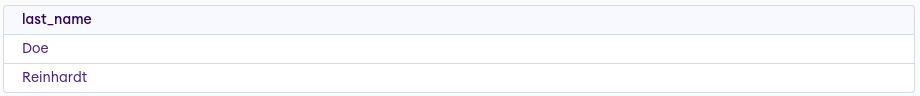

Intersect:

SELECT last_name
FROM Customers
WHERE first_name = "John"
 
INTERSECT
 
SELECT last_name
FROM Customers
WHERE first_name = "Betty"

Except:

SELECT last_name
FROM Customers
WHERE first_name = "John"

EXCEPT

SELECT last_name
FROM Customers
WHERE first_name = "Betty"

General procedure:

• Generate a Cartesian product of the relations in the from clause (puts the same name if unique else does tablename.attrname, the unique name can also be referred using the tablename.uniquename)
• Apply the predicates specified in the where clause
• For each tuple in result, output the attributes in the select clause (note: this sequence is what result of an SQL query should be, not how it should be executed)

Modifications:

Insertion:

INSERT INTO Customers
VALUES (10, "Ram", "Gopal", 15, "Nepal");

	must be in order but for any order:
	insert into course(title, course_id, credits, dept_name)
	values ('Database Systems', 'CS-437, 4, 'Comp. Sci')
	
	> Make students in Music who has earned more thatn 144 creidt hours an instructor in the Music department with a salary of 18000
	
	insert into instructor
		select ID, name, dept_name, 18000
		from student
		where dept_name = 'Music' and total_cred > 144;
	
	(Make sure to check select before insert)
	
	insert into <table name>
	tuples list goes here...
	values (...) or tuples themselves
	
Delete:
	-can only delete whole tuples, cannot delte values on only particular attributes
	
	delete from r
	where P;
	
	(works only on one relation)
	
	
Updates:

 	update instructor
	set salary = salary*1.05;
	where salary < 70000;
	
	multiple cases: (try to use above onlly)
	
	update instructor
	set salary = case
			when pred1 then result1
			when pred2 then result2
			...
			when predn then resultn
			else result0
		     end
	
	eg:
	
	update instructor
	set salary = case
			when salary <= 100,000 then salary*1.05
			else salary*1.03
		     end
	
SQL PRACTICAL THINGS: (BUT BEFORE PRACTISE WRITING QUERIES NOW)










Views:
	-Is a virtual table is the result of a stored query which is queried in the same manner as a persistent object
	-May wish to create a personalized collection of relations that is better matched to a certain user's intuition of the structure of the enterprise
	-Use SQL authorization mechanism to restrict access to relations
	-Why not store permanently? if we did so, and the underlying data in the relations changed, the stored query results would then no longer match the result of reexecuting the query on the relations
	
	Syntax: create view v as <query expression>;

	-Example:
		create view faculty as
			select ID, name, dept_name
			from instructor;
	is not precomputed and stored, instead the database system stores the query expression associated with the view relation
	
Materialized views:
	-Certain database system allow view relations to be stored in disk, making sure that if actual relations used in the view definition change, the view is kept up=to-date, such views are called materialized views
		>Views are used when data is to be accessed infrequently and the data in a table gets updated on a frequent basis. In contrast, Materialized Views are used when data is to be accessed frequently and data in table not get updated on frequent basis.
	-Applications that demand fast response to certain queries that compute aggregates over larget relations can benefit greatly by creating materialized views correspondin to the queries
	-Benefits to queries from the materialization of a view must be weighed against the storage costs and the added overhead for updates
	-SQL does not define a standard way of specifying that a view is materialized but many database systems provide their own SQL extensions for this task
	
Update of a view:
	-Views present serious problems if we express insertions, deletions or updates with them, as that a modification to the database expressed in terms of a view must be translated to a modification to the actual relations in the logical model of the database
	-In the faculty view:
		insert into faculty
			values ('3023', 'Green', 'Music');
	reasonable possibilities are:
		- Reject the insertion, and return an error message to the user
		- Insert (..., null) into the instructor relation
	-Because of problems such as these, modifications are generally not permitted on view relations, except in limited cases
	
	
SEGWAYS HERE:
	-QBE	
	
INTEGRITY CONSTRAINTS:
	-Ensures that changes made to the database by authorized users do not result in a loss of data consistency
	-In constrast, security constraints guard against access to the database by unauthorized users
	-Guards against accidental damage to the database
	-Examples:
		An instrcutor name cannot be null
		No two instructor can have same instructor ID
		Every deparment name in the course relation must have a matching department name in the department relation
	-Usually identified as part of database schema design process and declare as part of the create table command used to create relations
	-Can also be added to an existing relation by using the command alter table, if relation satisfies, the constraint is added to the relation, else rejected.
	
1. Domain constraints:
	-Enforces specific rules on the data that can be stored in a particular column or attribute of a database table
	- domains garauni such as int, char(10) varchar(10) numeric(12,2), text
	- not null
	- check at last as:
		check (semester in ('Fall', 'Winter', 'Spring', 'Summer'))

2. Entity integrity constraints:
	-unique (Aj, ... Am) says that the attributes form a superkey (but they could be null unless specially specified)
	-primary key (Aj1, ..., Ajm): requres to be nonnull and unique


3) Referential integrity:
	-Ensures that a value that appears in one relation (the referencing relation) for a given set of attributes also appears for a certain set of attributes in another relation (the referenced relation)
	-Foreign keys are a form of referential integrity constraint where the referenced attributes form a super key of the referenced relation
	-SQL DDL:
		foreign key (dept_name) references deparment
	
	>specifies that for each course tuple, the department name specified in the tuple must exist in the deparment relation
	>Without this constraint, it is possible for a course to specify a nonexistent deparment name
	>By default, in SQL a foreign key refernences the primary-key attriutes of the referenced table
	>Also, supports a version of the refernces clause where a list of attributes of the referenced relation can be specified explicitly
		foreign key (dept_name) references deparment(dept_name)
	>When a referential-integrity constraint is violated, the normal procedure is to reject the action that cause the violoation (the transaction performing the update action is rolled back)
	>However foreign key clause can specify that if a delte or update action on the referneced relation violates the constraint, then, instead of rejecting the action, the system must take steps to change the tuple in the referencing relation to store the constraint
	
	create table course
	(...
	foregn key (dpet_name) refernces department
		on delete cascade
		on update cascade
	
	[foregin key lel chai candidat ekey lai refrence garnu parxa bhanni sunna ma aako xa]
	
	Because of the clause on delete cascade associated with the foreign key declaration, if a delete of a tuple in deparment results in this referential-interigy constraint being violated, the system does not reject the delete, instead the delete cascades to the course relation, deleting ht tuple that refres to the deparment that was deleted


VIOLATION: Integrity constraint violation during a transaction:
	-Transactions may consist of several steps, and integrity constraints may be violated temporarily after one step, but a later step may remove the violation
	-The SQL allows intially deferred to be added to a constraint specificaiton; the constraint would hen be checked at the end of a trancaction and not at intermediate steps
	>Can altenratlively specified as deferrable, whcih means it is checked immediatley by default but can be deferred when desired

	
Triggers:
	-A trigger is a statement that the system executes automatically as a side effect of a modification to the database such as insertion, modification or deletion of data in a table
	-Allows to define custom code that is automatically executed before or after a particular event, providing a powerful way to enforce business rules, automate tasks, and implement complex logic in your database
	-To define a trigger, we must:
	
	1)Specify when a trigger is to be executed, which is broken up into an event that causes the trigger to be checked and a condition that must be satisfied for trigger execution to proceed
	2)Specify the actions to be taken when the trigger executes

	Uses:
	-Useful for alerting humans or for starting certain tasks automatically when certain conditions are met
	-Triggers can be used to implement certain integrity constraints that cannot be specified using the constraint mechanism of SQL
	-Example: 
		Say a employee table with columns id name salary and deparment, create a trigger that automatically updates the salary column for a given employee whenver there deparment column is change
		
		CREATE TRIGGER update_salary
		AFTER UPDATE on employees
		FOR EACH ROW
		BEGIN
			IF NEW.deparment <> OLD.deparment THEN
				UPDATE employees SET salary = 100,000 WHERE id = NEW.id;
			END IF;
		END;
		

Indexes:
	-Many queries reference only a small proportion of the records in a file, like finding all instructors in the Physics deparment
	-An index on an attribute of a relation is a data structure that allows the database system to find those tuples in the relation that have a specified value for that attribute efficiently, without scanning through all the tuples of the relation
	-For example, if we create an index on attribute dept name of relation instructor, the database system can find the record with any specified dept name value, such as “Physics”, or “Music”, directly, without reading all the tuples of the instructor relation.
	-Can also be created on a list of attributes
	
	>Indices are important for efficient processing of transactions, including both update transactions and queries, also important for efficient enforcement of integrity constraints such as primary-key and foreign-key constraints
	>Without indices, every query would end up reading the entire contents of every relation that it uses; doing so would be unreasonably expensive for queries that only fetch a few records
	>The database system can decide automatically what indices to create, however because of the space cost of indices, as well as the effect of indices on update processing, it is not easy to automatically make the right choices about what indices to maintain
	>Though not part of SQL syntax:
		
	create index <index-name> on <relation-name> (<attribute-list>);
	
	create index dept_index on instructor (dept_name);
	
	-When a user submits an SQL query that can benefit from using an idex, the SQL query processor automaically uses the index
	-If we wish to declare that the search key is a candidate key, we add the attribute unique to the index definition
	

	Two kinds of indexes:
		1. Ordered indices: Based on a sorted ordering of the values
		2. Hash indices: Based on a uniform distribution of values across a range of buckets
		
	ORDERED INDICES:
		-The ordered indices gains fast random access to records in a file by maintaing an index structure in a sorted order for a particular search key, whose index entry consists of search-key value and pointers to one or more records with that value as their search-key value
		-The records in the indexed file may themselves be stored in some sorted order
		-A clustering index is an index whose search key also defines the sequential order of the file, the search key of a clustering index is often the primary key, although that is not necessarily so
		-Indices whose search key specifies an order different from the sequential order of the file are called nonclustering indices
		-Two types:
		
		1. Dense index:
			-An index entry appears for every search-key value in the file
			-In a dense clustering, the index record contains the search-key value and a pointer to the first data record with that search-key value, the rest of the records with the same search-key value would be stored sequentially after the first record
			-For dense nonclustering index, the index must store a list of pointers to all records with the same search-key value
			
		2. Sparse index:
			-An index entry appears for only some of the search-key values
			-Can be used only if the relation is stored in sorted order of the search key; that is, if the index is a clustering index
			-Each index entry contains a search key value and a pointer to the first data record with that search-key value
			-To locate a record, we find the index entry with the largest search-key value that is less than or equal to the search-key value for which we are looking, we start at the record pointed to by that index entry and follow the pointers in the file until we find the desired record
			
		-Example of how to get to the record 2222
	
		>Generally faster to locate a record if we have a dense index rather than a sparse index, however sparse indices have advantages over dense indces in that they require less space and they impose less maintainence overhead for insertions and deletions
		>A good compromise is to have a sparse index with one index entry per block
	
	
	
		Insertions:
		>First the system performs a lookup using the search-key value that appears in the record to be inserted:
		1. Dense indices:
			>If the search key value does not appear in the index, the system inserts an index entry with the search-key value in the index at the appropriate position
			>Otherwise if clustering index, then places the record being inserted after the other records with the same search-key values, if nonclustering then adds a pointer to the new record in the index entry
			
		2. Sparse indices:
			>(Assume that the index stores an entry for each block)
			
		Deletions:
	
	
	
		
	HASH INDICES:
		-Maintains a bucket to store one or more records, which are basically a linked list of disk blocks
		-Formally, let K denote the set of all search-key values and let B denote the set of all bucket addresses, a hash function h is a function from K to B
		-To insert a record with search key Ki, we compute h(Ki) which gives the address or pointer of the bucket for that record, we add the index entry for the record to the list at offset i
		-To perform a lookup on a search-key value Ki, simply compute h(Ki) then search the bucket with that address, since two search keys could have the same hash value, have to check the search-key value of every record in the bucket that the record is one that we want
		-Worst hash function maps all the search-key values to the same bucket; this makes access time proportinal to the number of search-key values in the file
		-An ideal hash function is uniform i.e. each bucket is assigned the same number of search-key values from the set of all possible values
		-Typical hash functions perform computation on the internal binary representation of the search-key, for example, the binary representation of all characters in a string could be added and the sum modulo the number of buckets
		-Bucket overflow can occur because of:
		1. Insufficient buckets: 
		2. Skew:
		-Choose number of buckets as nr/fr*(1+d) i.e. 120% percentage more rey tara yesle only 1 lai prevent garna sakxa:
		-Hash indexing where the number of buckets is fixed when the index is created, is called static hashing
		-Allowing incremental increase of buckets: dynamic hashing
		Example: Extendable hashing
			-youtube heram
	
	
	B-Trees:
		-
		
		
		
	

RELATIONAL DATABASE DESIGN: (tradeoffs between efficiecny and redundancy, redundancy automatically implies consistency) > Goal of database design is to generate a set of relational schemas that allows us to store information without unnecessary redundancy, yet also allows us to retrieve information easily, accomplished by designing schemas that are in appropriate normal form > To determine whether a relation is in one of the desirable forms needs information about the real-world enterpise that we are modelling with the database > Example: Let’s use in_dep

	in_dep (ID, name, salary, dept_name, building, budget)
	
	instead of twos:
	
	instrutor (ID, name, dept_name, salary)
	deparment (dept_name, building, budget)
	
	which to use though?
	
	# Advantages:
		- Some queries can be expressed using fewer joins
	# Disadvantages: 
		- It stores budget amount redundantly
		- Runs the risk that some user might update the budge amount in one tuple but not all, thus consistency	
 
 > How to avoid such redundancy?
 	- A schema that exhibits repetition of information may have to be decomposed into several smaller schemas, though not all decompositions of schemas are helpful
	- NORMALIZATION garnu parxa bro
	

NORMALIZATION THEORY: 1) Decide if a given relation is in normal forms 2) If not then we decompose it into a number of smaller relation schemas, each of which is an appropriate normal forms

Advantages of normalization: -Is the process of structuring relational database in accordinate with a series of normal forms in order to reduce reduancng and improving data integirty: -Example yeta halda thik hola 1. Ensuring data integrity: -Enforces integrity constraints 2. Elimitaing data redundancy: -Removes duplicates as budget is duplicate there 3. Insertion, deletion and update anamolies: -Cannot insert a new deparment without an instructor -If delete an instructor who is the only one working in a deparment, then deparment info is lost -if update a deparment info then update all the tuples containing it 4. Database performance: -Breaking down a large table into smaller, each containing a subset of data elements, normalization makes it easier to retrieve data quickly and efficiently 5. Database maintainence: -Smaller tables makes it easier to add or remove data elements without affecting other parts of the schema

LOSSLESS DECOMPOSITION:
	(comment: schema vs relation ta yaad xa ni? schema bhaneko design jastai ho bro, instructor(a, b, c) yo schema ho ra yesto data aayo bhane chai yo relation hunxa, in other words schema bhaneko headings haru ho relation bhaneko data)
	
	- Let R be a relation schema and let R1 and R2 form a decomposition of R i.e. as sets of attributes R = R1 \cup R2
	- Loss of information occurs if it is possible to have an instance of relation r(R) that includes information that cannot be represented if instead of the instance of r(R) we must use instances of r1(R1) and r2(R2).
	- Formally, is lossless, if for all legal database instances, relation r contains the same set of tuples as the result of the following SQL query,
		select *
		from (select R1 from r)
			natural join
		     (select R2 from r)
		
		<in relational algebra:>
		
		Pi_{R1}(r) natural join Pi_{R2}(r) = r
		
	- Conversely, is lossly if,
		r \prop_subset Pi_{R1}(r) natural join Pi_{R2}(r)
	- Counterintuitive as we have more tuples but less informatino as decomposed version is unable to represent the absence of a connections, and absence of a connection is indeed information
	

(arko tarika bata lossless decomposition) KEYS AND FUNCTIONAL DEPENDENCIES: -Most real-world constraints an be represented formally as keys, or as functional dependencies -As superkey is a set of attributes that uniquely identifies an entire tuple, a functional dpendency allows to express constraints that uniquely identify the values of certain attributes

	# Given r(R), a subset of K of R is a superkey of r(R) if, in any legal instance of r(R), for all pairs t1 and t2 of tuples in the instance of r if t1 != t2, then t1[K] != t2[K], i.e. no two tuples in any legal instance of relation r(R) may have the same value on attribute set K
	
	(candidate key ni define garihalam)
	Given r(R), a subset of K of R is a candidate key of r(R) if it is a superkey of r(R) and no proper subset of K is a superkey of r(R), i.e. a candidate key is a minimal superkey that uniquely identifies each tuple in the relation.
		
	(foreign key ni haldihaaley hai yesaima)
	Given two relation schema r1(R1) and r2(R2) then a foregin key from r1 to r2 is a set of attributes K in R1 such that for every tuple t1 in R1, the value of the attribute in K uniquely identifies a tuple t2 in R2 such that t1[K] = t2[K] and the attributes in K must be a superkey of R1 i.e. no two tuples in any legal instance of R1 may have the same value on attribute set K
	
	(primary key lai kina chodni)
	A primary key is a chosen candidate key that is used as a main means of uniquely identify tuples in a relation
		
	# Let \alpha and \beta be attributes of relation schema r(R) then the instance r(R) satisfies the functional dependency alpha -> beta if for all pairs of tuples t1 and t2 in the instance such that t1[\alpha] = t2[\alpha], it is also the case that t1[\beta] = t2[\beta]
	(means that yedi t1 ra t2 ma euta attribute same bhayo bhane arko attribute ni same hunai paryo, in other words, beta component is determined by the alpha component)
		
-In this language, we say that K is a superkey for r(R) if the functional dependecny K -> R holds on r(R) (meaning that if K is same for two tuples then everything is same)
-Some dependencies are trivial such as beta subset of alpha then alpha -> beta is trivial
-Given a set of functional dependencies F holds on a relation r(R) it is possible to infer that certain other functional dependencies hold, say F+ is closure that includes all such dependencies

>For eg: given a schema r(A,B,C), if functional dependencies A -> B and B-> C hold on r, can infer the functional dependency A -> C must also hold on r
	
	

LOSSSLESS DECOMPOSITION IN TERMS OF DEPENDENCIES: -R1 and R2 form a lossless decomposition if at least one of the following dependencies is in F+: R1 \cap R2 → R1 R1 \cap R2 → R2

(i.e. if R1 cap R2 forms a superkey for either R1 or R2 then is lossless)
	
-Example: 
	Considering the schema:
		in_dep (ID, name, salary, dept_name, building, budget)
	decomposed into:
		instructor (ID, name, dept_name, salary)
		department (dept_name, building, budget) 
	
	Here,
		dept_name -> dept_name, building, budget
	
	so, is a lossless decomposition
	
-NOTE: For decomposition into multiple schemas at once, the test is more complicated, while the test for binary decomposition is clearly a sufficient condition for lossless decomposition, it is a necessary condition only if all constraints are functional dependencies
(aru constraint exist such as multivalued dependencies)

-Suppose we decompose r(R) into r1(R1) and r2(R2) where R1 cup R2 -> R1 then following SQL constraints must be imposed on the decomposed schema
	> R1 cap R2 is the primary key of r1
	(enforces the functional dependency)				
	> R1 cap R2 is a foregin key from r2 referencing r1
	(ensures that each tuple in r2 has a matching tuple in r1, without which it would not appear in the natural join of r1 and r2)
		
 -If r1 or r2 is decomposed further, as long as the decomposition ensures that all attributes in R1 cap R2 are in one relation, the primary or foreign key constraints on r1 or r2 would be inherited by that relation
		

Some special dependencies: 1. Trivial: 2. Partial: A functional X→Y is a partial dependecncy if some attribute A of X can be removed from X and the dependnecy still holds i.e (X-{A}) → Y

NORMAL FORMS:

1. Boyce-Codd Normal Form:

   -Eliminates all redundancy that can be discovered based on functional dependencies (though other types of redundancy maybe remaining)

   A relation schema R is in BCNF with respect to set F of functional dependencies if, for all functional dependencies in F+ of the form \alpha → \beta, where \alpha \subset R and \beta \subset R, at least one of the following holds

   1. \alpha → \beta is a trivial functional dependency (i.e. \beta \subset \alpha)
   2. \alpha is a superkey for scheme R

   EXAMPLE:

   An example of relational schema that is not in BCNF is in_dep, since dept_name → budget holds in in_dep but dept_name is not a superkey (a department may have a number of different instructors)

   The decomposition of the in_dep schema is in BCNF: ID → name, dept_name, salary; dept_name → building, budget

   General rule for decomposing schemas that are not in BCNF: > Let R be a schema that is not in BCNF, then there is at least one nontrivial functional dependency \alpha → \beta such that \alpha is not a superkey for R, replace R with two schemas: 1) (\alpha \cup \beta) 2) (R - (\beta - \alpha)) > Example: \alpha = dept_name, \beta = {building, budget} then new schemas are: - (dept_name, building, budget) - (ID, name, dept_name, salary)

    > When we decompose a schema that is not in BCNF, it may be that one or more of the resulting schemas are not in BCNF, in such cases, further decomposition is required
    
   

   Note: -The BCNF design may not permit the enforcement of the functional dependencies without a join (there is no schema that includes all the attributes appearing in the funcional dependency), so the design is said to be not dependency preserving -Worth noting that SQL does not provide a way of specifying functional dependencies

   WHAT IS DEPENDENCY PRESERVATION? -Let F be a set of functional dependencies on a schema R, and let R1, R2, … Rn be a decomposition of R, the restriciton of F to Ri is the set Fi of all functional dependencies in F+ that include only attributes of Ri (restrictions F1 .. Fn ma chai aafno decomposition wala relation ko matra columns hunxa) -Let F’ = F u F2 u .. u Fn, F’ is a set of functional depdencies on schema R, but in general F’ != F, even though it may be that F’+ = F+, if true then every dependency in F is logically implied by F’ -We say that a decomposition having property F’+ = F+ is a dependency-preserving decomposition -Given R(A,B,C) with functional dependencies F = {A→B, B→C} can be decomposed in two different ways: 1. R1 = (A,B), R2 = (B,C) FD1 = {A→B}, FD2 = {B→C} Here, {FD1 u FD2}+ == F+ >Dependency preserving

    2. R1 = (A,B), R2 = (A,C)
    	FD1 = {A->B}, FD2 = {A->C}
    	Here, {FD1 u FD2}+ != F+
    	>Not dependency preserving
   

   HOW TO FIND CLOSURE OF ATTRIBUTES UNDER F? -(hamlai each attributes ko closure find garnu parxa hai say alpha)

    result := alpha
    repeat
    	for each functional dependency beta -> gamma in F do
    		begin
    			if beta \subset result then result := result u gamma
    		end
    	until (result does not change)
    
   

2. Third Normal Form:

   -Relaxes the constraints of requiring that all nontrivial dependencies of the from \alpha → \beta, where \alpha is the superkey, by allowing certain nontrivial functional dependencies whose left side is not a superkey

   A relation schema R is in third normal form with respect to a set F of functional dependencies if, for all functional dependencies in F+ of the form \alpha → \beta, where \alpha \subset R and \beta \subset R, at least one of the following holds:

   1. \alpha → \beta is a trivial functional dependency (i.e. \beta \subset \alpha)
   2. \alpha is a superkey for scheme R
   3. Each attribute A in \beta - \alpha is contained in a candidate key for R

   say that a single candidate key must contain all the attributes, may be contained in a different candidate key)

   The third alternative represents a minimal relaxation of the BCNF conditions that hellps ensure that every schema has a dependency-preserving decomposition into 3NF

BCNF VS 3NF: 3NF adv: Always possible to obtain a 3NF design without sacrificing losslessness or dependency preservation 3NF dis: May have to use null values to represent some of the possible meaningful relationships among data items, and there is the problem of repetition of information

Hence, goals of database design:
	1. BCNF
	2. Losslessness
	3. Dependency preservation
	
-Since, not possible to satisfy all three, may be force to choose between BCNF and dependency preservation (with 3NF)

DECOMPOSITION USING MULTIVALUED DEPENDENCIES: - Some schemes, even though they are in BCNF, do not seem to be sufficiently normalized, they still suffer from the problem of repition of information, say a variation where instructor may be associated with multiple departments inst (ID, dept_name, name, street, city)

is a non-BCNF schema because of the functional dependency:

	ID -> name (where ID iss not a key for inst)
	
Following BCNF decomposition:
	 r1 (ID, name)
	 r2 (ID, dept_name, street, city)
	 
Despite r2 being in BCNF, there is redundancy, is repeat the address information of each residence of an instructor once for each deparment with which the instructor is associated, further decompose (no constraint?)

	r21 (ID, dept_name)
	r22 (ID, street, city)

To deal with this, is a new form of constraint, called a multivalued dependency, which defines a new normal form called 4NF

>Functional dependencies rule out certain tuples from being in a relation, if A -> B then we cannot have two tuples with same A but different B values. 
>Multivalued do not rule out the existence of certain tuples, instead they require that other tuples of a certain form be present in the relation
>Functional dependencies are referred to as equality-generating dependencies, and multivalued dependencies are referred to as tuple-generating dependencies
- Let r(R) be a relation schema and let \alpha \subset R and \beta \subset R, the multivalued dependency:
		 \alpha ->-> \beta
holds on R if, in any legal instance of relation r(R), for all pairs of tuples t1 and t2 in r such that t1[\alpha] = t2[\alpha], there exist tuples t3 and t4 in r such that
		t1[\alpha] = t2[\alpha] = t3[\alpha] = t4[\alpha]
		t3[\beta] = t1[\beta]
		t3[R-\beta] = t2[R-\beta]
		t4[\beta] = t2[\beta]
		t4[R-\beta] = t1[R-\beta]
		
-Intuitively, the relationship between \alpha and \beta is independent of the relationship between \alpha and R-\beta
-Take r2 schema:
	>The relationship between an instructor and his address is independent of the relationship between that instructor and a deparment
-So we need, ID ->-> dept_name or ID ->-> street, city to hold

OTHER NORMAL FORMS:

1. 1NF: -A relation schema r(R) is in first normal form if the domains of all attributes of R are atomic that is, they are indivisible units -ER model allows entity sets and relationships to have attributes that have some degree of substructure, which are elimiated when creatingt tables from ER designs to maintain 1NF -For composite attributes, let each component be an atribute in its own right -For multivalued attributes, create one tuple for each item in a multivalued set -Example: >A set of names is an example of a non-atomic value, if a relation employee included an attribute phone number whose domain elements are sets of integers, the schmea would not be in first normal form >| Employee_ID INT | Children_Names SET OF INT |

2. 2NF: -A functional dependency alpha → beta is called a partial dependency if there is a proper subset gamma of alpha such that gamma → beta; we say that beta is partially dependent on alpha. -A relation schema r(R) is in 2NF if each attribute A in R meets one of the following criteris: >It appears in a candidate key >It is not partially dependent on a candidate key

   (primary key single attribute bhayo bhane ta 2NF tesai bhaihalyo)

QUERY PROCESSING: -Refers to the range of activities involved in extracting data from a database, includes 1) Parsing and translation: -Translation of queries in high-level database languages into expressions that can be used at the physical level of the file system 2) Optimization: -A variety of query-optimizing transformations, 3) Evaluation: -Actual evaluation of queries

DETAILS:

PARSING AND TRANSLATION:
-The first stage of processing processing is to translate the query into a usable form, SQL is suitable for human use, but ill suited to be the system's internal representation of a query, more useful internal representation is one based on the extended relational algebra
-Process is similar to the work performed by the parser of a compiler
-After verifying the syntax of the user's query, the system constructs a parse-tree representation of the query, which it then translates into a relational-algebra expression (if the query was expressed in terms of a view, the translation phase also replaces all uses of the view by the relational-algbera that defines the view)
		
	Consider the query:
		select salary
		from instructor
		where salary < 75000;
		
	this query can be translated into either of the following relational-algebra expressions:
		
	\sigma_{salary<7500}(\Pi_{salary}(instructor))
	\Pi_{salary}(\sigma_{salary<7500}(instructor))
		
	which can then be executed by one of several different algorithms
		
-To specify fully how to evaluate a query, we need not only to provide the relational algebra expression, but also to annotate it with instructors specifying how to evaluate each operation
	d>For example to implement preceding query, we can search every tuple in instructor to find tuples with salary less than 75000; if a B+-tree index is avaialable on the attribute salary, we can use the index o locate the tuples
-A relational-algebra operation annotated with instructors on how to evaluate it is called an evaluation primitive
-A sequence of primitive operations that can be used to evaluate a query is a query-execution plan or query-evaluation plan
-The query-execution engine takes a query-evaluation plan, executes that plan, and returns the answers to the query
-It is the responsibility of the system to construct a query-evaluation plan that minimizes the cost of query evaluation; this task is called query optimization

Note: sequence of steps described for processing a query is representative; not all databases exactly follow those steps, for instance, instead of using the relational-algebra representation, several databases use an annotated parse-tree representation based on the structure of the given SQL query


OPTIMIZATION:
-As there are multiple evaluation plans for a query, and it is important to be able to compare the alternatives in terms of theri estimated cost, and choose the best plan
-The cost of query evaluation can be measured in terms of a number of different resources, including disk accesses, CPU time to execute a query, and, in parallel and distributed database systems, the cost of communication

<Here goes how each part of query are estimated and how individual relational operation are performed: okay join ko heram na ta>

1. Nested loop join:
	-
	
2. Block nested loop join:
	-

EVALUATION:
-The simple way to evaluate an expression is simply to evaluate one operation at a time, in an appropriate order where the result of each evaluation is materialized in a termporary relation for subsequent use. A disadvantage to this approach is a need to construct materialized relation for subsequent use
-An alternative approach is to evaluate several operations simultaneously in a pipeline, with the results of one operation passed on to the next, without the need to store a temporary relation


MATERIALIZATION:

-Consider the expression:
	Pi_{name}(sigma_{building="Watson"}(department) natural join instructor)
	
-If we apply the materialization approach, we start from the lowest-level operations in the expression (at the bottom of the tree)
-The inputs to the lowest level operations are relations in the database
-In the lowest level, there is only one such operation; the selection operation on deparment, which operations are executed using the individual algorithms, and results are stored in temporary relations
-Can use these temporary relations to execute the operations at the next level up in the tree, where the inputs now are either temporary relations or relations stored in the database
-The join can now be evaluated, creating another temporary relation
-By repeating the process, we will eventually evaluate the operation at the root of the tree, giving the final result of the expression, in our example, the final result is by executing the projection operation at the root of the tree, using as input the temporary relation created by the join
-This is called materialized evaluation, since the results of each intermediate operation are created (materialized) and then are used for evaluation of the next-level operations

>The cost of materialized evaluation is not simply the sum of costs of the operations involved, as we ignored the cost of writing the result of the operation to disk
>Assume that the records of the disk accumulate in a buffer, and when buffer is full, they are written to disk
>The number of blocks written out, br, can be estimated as nr/fr, where nr is the estimated number of tuples in the result relation r and fr is the blocking factor of the result relation, i.e. the number of records of r that will fit in a block
>Some disk seeks may be required, since the disk head may have moved between successive write, the number of seeks can be estimatd as ceil(br/bb) where bb is the size of the output buffer (measures in blocks)

Double buffering: (using two buffers, with one continuing execution of the algorithm while the other is being written out) allows the algorithm to execute more quickly by performing CPU activity in parallel with IO activity, the number of seeks can be reduced by allocating extra blocks to the output buffer and writing out multiple blocks at once


PIPELINING:

-Can improve query-evaluation efficiency by reducing the number of temporary files that are produced which is achieved by combinding several relational operations into a pipeline of operations, in which the results of one operation are passed along to the next operation in the pipeline
-Example:
	Pi_{a1, a2}(r natural join s)
if materialization were applied, evaluation would involve creating a temporary relation to hold the result of the join and then reading back in the result to perform the projection
-Instead combining them: when the join operation generates a tuple of its result, it passes that tuple immediately to the project operation for processing
-In the earlier example, all three operations can be placed in a pipeline, which passes the results of the selection to the join as they are generated, in turn, it passses the results of the join to the projection as they are generated

Benefits:
	1) Eliminates the cost of reading and writing temporary rleations, reducing cost of query evaluation
	2) It can start generate query results quickly, if the root operator of a query-evaluation plan is combined in a pipeline with its inputs, this can be quite useful if the results are displayed to a user as they are generated, since otherwise there may b a long delay before the user sees any query results
	
Implementation of pipelining:

1) Demand-driven pipeline
	-The system makes repeated requests for tuples from the operation at the top of the pipeline (comment: tree ko top le request pathauxa jun propagate hudai tala samma aauxa)
	-Each time that an operation receives a request for tuples, it computes the next tuple (or tuples) to be returned and then returns that tuple
	-If the inputs of the operation are not pipelined, the next tuple(s) to be returned can be computed from the input relations, whilie the system keeps tract of what has been returned so far. 
	-If it has some pipelined inputs, the operation also makes requests for tuples from its pipelined inputs
	-Using the tuples received from its pipelined inputs, the operation computes tuples for its output and passes them up to its parent
	
2) Producer-driven pipeline
	-Operations do not wait for requests to produce tuples, but generate the tuples eagerly
	-Each operation in a producer-driven pipeline is modelled as a separate process or thread within the system that takes a stream of tuples from its pipelined inputs and gnerates a stream of tuples for its output
	

QUERY OPTIMIZATIONS: -To find the least costly query-evaluation plan, the optimizer needs to generate alternative plans that produce the same result as the given expression and to choose the least costly one -Involves three steps 1. Genearting expressions that are logically equivalent to the given expression 2. Annotating the resultant expressions in alternative ways to generate alternative query evaluation plans 3. Estimating the cost of evaluation plan, and choosing the one whose estimated cost is the least

-To implement the first step, the query optimizer must generaate expressions equivalent to a given expression which it does so by means of equivalence rules that specify how to transform an expression into a logically equivalent one

Equivalence rules:
	
1. Selection operations are commutative:
	sigma_(theta1)(sigma_(theta2)[E])
	
3. Theta join operations are commutative
	...

3. Selection distributes over the theta join when all the attributes in selection condition involve only the attributes of one of the expressions:
	sigma_{theta} (E1 natural join E2) = (sigma_{theta} (E1)) natural join (E2) 

	
Ex:
	pi_name (sigma_{course=DBMS} (teaches natural join instructor))
	
	is equivalent to
	
	pi_name (sigma_{couse=DBMS} teaches natural join instructor)

	is equivalent to
	
5. Join ordering: (reduces the size of temporary storages)

	pi_name (instructor natural join sigma_{course=DBMS} teaches)


Evaluation plans:

-Generation of expressions is onl part of the query-optimization process, since each operation in the expression can be implemented with different algorithms
-An evaluation plan defines exactly what algorithm should be used for each operation, and how the execution of the operations should be coordinated
-A cost-based optimizer explores the space of all query-evaluation plans that are equivalent to the given query, and chooses the one with the least estimated cost, can estimate its cost using statistics estimation techniques
-However, cost-based optimization with arbitrary equilvanece rules is fairly complicated, exploring the space of all possible plans may be too expensive for complex queries
-Eg:
	Consider finding the best join-order for r1 natural join r2 ... rn
	
	-There are (2(n-1))!/(n-1)! join orders for above expressions, with n = 10 the number is greater than 17.6 billion
	-However using dynamic programming, the least-cost join order for any subset of (r1, ... rn} is precomputed only once and stored for future use
	-Which reduces the time complexity to O(3^n) which with n = 10 is 59000
	
-Although the cost of query optimization can be reduced by clever algorithms, the number of different evaluation plans for a query can be very large, and finding the optimal plan from this set requires a lot of computational effors, hence optimizers use heuristics to reduce the cost of optimization
-Example:
	>Perform selection operations as early as possible
-A heurestic optimizer would use this rule without finding out whether the cost is reduced by this transformation
-Is heuristic because it usually, but not always, helps to reduce the cost, for example, in an expression sigma_theta(r natural join s), where theta attributes refers to only attributes in s. Selection can certainly be performed before join but if there is an index on the join attributes of s, but no index on the attributes of theta, then it is probably a bad idea to perform the selection early
-Others:
	>Perform projections early
	>Sytem R only considers left-deep join orders which are particularly convient for pipelined evaluation
	
	
	
	
	
	
	
	
	
	
	
	
	
	
	
	
	
	
	
	
	
	
	
	
	
	
	

NEED to study again these shits because of exams:

Data storage structures: -Magnetic disks as well as SSDs are block strucured devices, that is, data are read or written in units of a block, ins contrast, databases deal with records, to ensure efficient access, as well as to support recovery from failures, databases must continue to be aware of blocks -In a relational database, tuples of distinct relations are generally of different sizes, one approach to mapping the database to files is to use several files and to store records of only one fixed length in any file -An alternative is to structure our files so that we can accomodate multiple lenghts for records; however, files of fixed-length records are easier to implement than are files of variable length records

1. Fixed-length records:
	-Instead of allocating a variable amount of bytes for the attributes, allocate the maximum number of bytes that each attribute can hold, say 53 bytes long
	-Simple approach is to use first 53 bytes for the first record, the next 53 bytes for the second and so on
	
	Problems:
		-Unless the block size happens to be a multiple of 53, soem records will cross boundaries, that is, part of the record will be stored in one block and part in another
		Ans: Allocate as many records to a block as would fit entirely in the block
		-Difficult to delete a record from this structure, the space occupied by the record to be deleted must be filled with some other record of the file
		Ans: 
		-Move the record that comes after it into the space formely occupied by the deleted record, and so
		-Maintain a free list of available record space
		
2. Variable-length records:
	-Variable-length records arise in database systems due to several reasons, most common reason is the presence of variable length fileds, such as strings, other reasons include record types that contain repeating fields such as arrays or multisets
	-Different techniques for implementing variable-length records exist, two different problems must be solved by any such technique:
		i. How to represent a single record in such a way that indiviual attributes can be extracted easily, even if they are of variable length
		Ans: Has two parts: an initial part with fixed-length information, whose structure is the same for all records of the same relation, followed by the conents of variable-length attributes. Fixed length attributes such as numeric values, dates are allocate as many bytes as required to store their value. Variable-length attributes such as varchar are represented in the initial part of the record by pair (offset, length), where offset denotes where the data for that attriute begins within the record, and length is the length in bytes of the variable-sized attribute
	
		ii. How to store variable-length records within a block, such that records in a block can be extracted easily
		Ans: Slotted-page structure is commonly used. There is a header at the beginning of each block, containing the information: number of record entries in the header, end of free space in the block, an array whose entries contain the location and size of each record. The actual records are allocated contiguously in the block, starting from the end of the block. If a record is deleted, the space that it occupies is freed, and its entry is set to deleted. Further, the records in the block before the delted records are moved, so that the free space created by the deletieon gets ocupied and all free space is again between the final entry in the header array and the first record. Can be moved as there be no pointers that point directly to the records
		







TRANSACTIONS
-A transaction consits of a sequence of query and/or update statements that form a logical unit of work where the database ensures that the entire transaction executes or none of it does
-In many SQL implementations, including MySQL and PostgreSQL, by default each SQL statement is taken to be a transaction on its own, and it gets committed as soon as it is executed, such automatic commit of individual SQL statements must be turned off if a transaction consisting of mulitple SQL statements needs to be executed
-Many databases support the commmand set autocommit off	

(Transactions)

ADVANCED SHITS THEY SAY:

Parallel systems; -Improves processing and IO speeds by using a large number of computers in parallel -A ccourse-grain parallel machine consists of a small number of powerful processors; a fine-grain machine uses thousands of small processors -The transaction requirements of organizations have grown with the increasing use of computers, the growth of WWW has created many sites with million of viewers, and increasing amounts of data collected from these viewers has produced extremely large databases at many companies -(speed up resources badhey sanga linear hunu parne tara hudania bhanni kura dekhauni) -Architecture haru: shared memory, shared disk, shared nothing and hybrid -shared garda kheri aauni problems jastai race conditions, cache coherecny

Distributed systems: (euta site ra arko site lai cloud bata connect gareko figure) -The databsase is stored on nodes located at geographically separated sites -Nodes in a distributed system communicate with one another through various communicaiton media, such as high speed private networks or the internet -Differences between shared nothing parallels or features bhanda ni bhayo 1. Distributed databases have sties that are geographically separated, as a result network conenctions have lower bandwidth, higher latency, and greater probabiliyt of failures, as compared to other networks within a single data center 2. Distrubted systems need to continue working even in the event of failure of an entire data center, to ensure high availability, requires replication of data across geographically separated data centers, to ensure that a common natural disaster does not affect all the data centers 3. Nodes in distributed database tend to vary more in size and function, whereas parallel databases tend o have nodes that are of similary capacity 4. Need to differentiate between local and glocal transactions, a local is one that accesses data only from nodes where the transaction was initiated, glocal on the other hand, is one that either acceses data in a node from one at which the transactoin was initiated, or accesses data in several differnt nodes

HOMOGENEOUS:
	-Nodes share a common global schema although some relations may be stored at some nodes, all nodes run the same distributed database management software and nodes actively coorporate in processing transactions and queries

HETERGENOUS:
	-In many cases a distributed database has to be consructed by linking together multple already existing database systems each with its own schema and possibly running different database management sfotware, the sites may not be aware of each other 

Vertical and horizontal fragmentation:

Special databases such as spatial and object oriented: Definitions Models Types Indexing Quering and indexing Applications Tools and platforms

Datawarehousing: -Large oranizations have a complex internal organization structure, and therefore different data may be present in different locations, or on different operational systems, or under different schemas -For example, manufacturing problem data and customer complaints may be stored in different database systems -Coorporate decision makers require access to information from multiple sources -A data warehouse is a repository or archive of information gathered from multiple sources stored under a unified schema, at a single site -Once gathered, the data are stored for a long time, permitting access to historical data, thus data warehouse provide the user a single consolidated interface to data, making decision support queries easier to write -Moreover, by accessing information for decision support from a data warehouse, the decision make ensures that online transaction processing systems are not affected by deciosn support workload

			by using a deadlock detection and recovery scheme