Simulation Undergrad

System:

A system is defined as an aggregation or assemblage of objects joined in some regular interaction or interdependence. Systems are of two types:

• Static system
• Dynamic system In static systems there are no changes over time where as in dynamic systems the interactions cause changes over time. Static models can only show the values that system attributes take where the system is in balanced. Dynamic models follow the changes over time that result from system activities.

The state of the system is to mean description of all entities, attributes, and activities as they exist at one point of time. The progress of the system is studied by the system following a change in the state of the system.

Example:

Consider a factory that make assembles parts for a product. Two major components of the factory system are the fabrication department that makes the part and the assembly department that produces the product. A purchasing department maintains & a shipping department dispatches the finished product. A production control department receives order & assigns work to the other department.

System modelling:

The model is the body of information about a system gathered for the purpose of studying the system. Since the purpose of the study will determine the nature of information that is gathered, there is no unique model of a system. Diferent models of the same system will be produced by different analysis interested in different aspects of the system or by the same analyst as his understanding of the system changes.

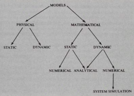
Physical models :

are the scaled down model of actual system, which has all the properties of the system, or at least it is as close to the actual system as possible. Now-a-days small models of cars, helicopters and aircraft are available in the market. These toys resemble actual cars and aircraft. They are static physical models of dynamic systems (cars, helicopters and aircraft are dynamic systems). The system attributes are represented by such measurements as voltage or the position of a shaft. The system activities are reflected in the physical laws that derive the models.

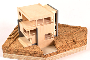
1. Static physical models:

   Static physical model is a scaled down model of a system which does not change with time. An architect before constructing a building, makes a scaled down model of the building, which reflects all it’s rooms, outer design and other important features. This is an example of static physical model. Similarly for conducting trials in water, we make small water tanks, which are replica of sea, and fire small scaled down shells in them. This tank can be treated as a static physical model of ocean.

2. Dynamic physical models:

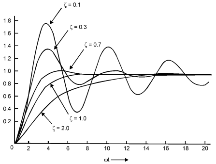
   Dynamic physical models are ones which change with time or which are functions of time. In wind tunnel, small aircraft models (static models) are kept and air is blown over them with different velocities and pressure profiles are measured with the help of transducers embedded in the model. Here wind velocity changes with time and is an example of dynamic physical model. A model of a hanging wheel of vehicle is another case of dynamic physical model discussed further.

   Consider an example of hanging wheel of a stationary truck and analyze its motion under various forces. Let a wheel of mass $M$, suspended in vertical direction, a force $F(t)$, which varies with time, is acting on it. Mass is connected with a spring of stiffness $K$, and a piston with damping factor $D$. When force $F(t)$ is applied, mass $M$ oscillates under the action of these forces. This model can be used to study the oscillations in a motor wheel.

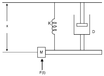   It can be shown that the motion of system is described by the following differential equation: $M\ddot{x}+D\dot{x}+Kx=KF(t)$

Mathematical models:

A physical model can be converted to a mathematical one. Most of the systems can in general be transformed into mathematical equations. These equations are called the mathematical model of that system. Since beginning, scientists have been trying to solve the mysteries of nature by observations and also with the help of Mathematics. Kepler’s laws represent a dynamic model of solar system. Equations of fluid flow represent fluid model which is dynamic.

1. Static mathematical models:

   A static model gives relationships between the system attributes when the system is in equilibrium. If the point of equilibrium is changed by altering any of the attributes values, the model enables the new values for all the attributes to be derived but does not show the way in which they changed to their new values.

   The supply and demand market model can be represented as a static mathematical model to analyze market equilibrium at a given point in time. In this model, the quantities of supply and demand are related to the price of a good or service, without explicitly modeling how these relationships evolve over time. The

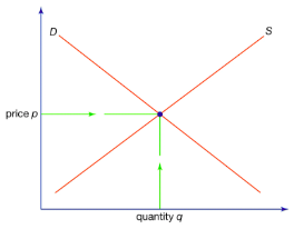   Since the relationships are have been assumed linear, the complete market model can be written mathematically as follows: $Q=a-bP$ S=c+dP$$$$S=Q The last equation states the condition for the market to be cleared; it says supply equals demand and, so, determines the price to which market will settle. The equilibrium market price, in fact, is given by the following expression: $P=\frac{a-c}{b+d}$

2. Dynamic mathematical models:

   The model of a stationary wheel equation is a dynamic mathematical model, as equations are function of time. This equation can be solved numerically with the help of Runge-Kutta method: $\frac{d^{2}x}{d{t}^2}+2\chi \omega \frac{dx}{dt}+{\omega }^{2}x={\omega }^{2}F(t)$where $2\chi \omega =\frac{D}{M}$ and ${\omega }^2=\frac{K}{M}$. Expressed in this form, solution can be given in terms of the variable $\omega t$

   

Simulation:

A simulation is the imitation of the operation of real-world process or system over time. Whether done by hand or on a computer, simulation involves the generation of an artificial history of a system and the observation of that artificial history to draw inferences concerning the operating characteristics of the real system.

The hanging wheel of a vehicle can be shown by numerical computations that the system does not oscillate when parameter $\chi \ge 1$. If it was possible to get analytical solution, one could easily find by putting $\chi =1$, that system does not oscillate. However, with the method of numerical techniques, one has to run the program for different values of $\chi$ and then find out that for $\chi \ge 1$, system is stable. Same is the case with simulation. One has to run simulation model number of time, to arrive at a correct output. Due to this reason, sometimes numerical computation is called simulation. But information derived numerically does not constitute simulation. Numerical computation only gives variations of one parameter in terms of other and does not give complete scenario with the time.

System simulation as the technique of solving problems by the observation of the performance, over time, of a dynamic model of the system.

Simulation is modeling and analyzing the behavior of complex systems by running experiments on model replicas of those systems.

When not to do simulation?

• When the problem can be solved by common sense
• or analytically
• If it is easier to perform direct experimentation
• If the costs exceed savings
• If the resources or time are not available

Monte-carlo simulation:

A Monte Carlo simulation is a computational technique that uses repeated random sampling to obtain numerical results, typically employed to model the probability of different outcomes in a process that cannot easily be predicted due to the intervention of random variables.

Given a rectangle for which we know the length $10\times 4$ units. It is split into two sections which are identified using different colors. What is the area covered by the black color? Due to the irregular way in which the rectangle is split, this problem cannot be easily solved using analytical methods. However, we can use Monte Carlo simulation to easily find an approximate answer. The procedure is as follows:

• Randomly select a location (point) within the rectangle
• If it is within the black area, record this instance a hit
• Generate a new location and follow 2
• Repeat this process 10,000 times

After using MC simulation a test 10,000 random points, we will have a pretty good average of how often the randomly selected location falls within the black area. We also know from basic mathematics that the area of the rectangle is 40 square units. Thus, the black area can be calculated by: $\text{Black area}=\frac{\text{number of black hits}}{10,000}\times 40\text{ square units}$

(these are for mathematical dynamic models:)

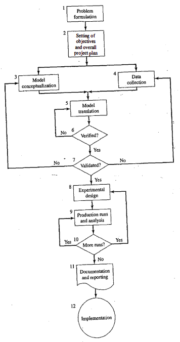
Steps in simulation study:

1. Problem formulation: clearly understood problem statement, provided by the policymakers

2. Setting of objectives and overall project plan: indicate the questions answered by the simulation

3. Model conceptualization: as much as art as science, involve users

4. Data collection: real data for validation

5. Model translation: computer programs

6. Verification:

7. Validation:

8. Experimental design:

9. Production run and analysis:

10. More runs?

11. Documentation and reporting?

12. Implementation:

Continuous simulation:

A continuous system is one in which the predominant activities of the system cause smooth changes in the attributes of the system entities. Modeling and simulation of various problems like pursuit evasion of aircraft, fluid flow, flight dynamics and so on come under continuous system simulation. Continuous system generally varies with time and is dynamic. One of the definitions of a discrete variable is that it contains at most finitely many of the values, in a finite interval on a real number line. Thus there can be certain portions on the number line where no value of discrete variable lies. But in the case of continuous variable, it has infinite number of values in a finite interval.

By continuous we mean uninterrupted, remaining together, not broken or smooth flowing. As per the definition given above there is no interval, how so ever small, on number line where a value of continuous variable is not there. If $f(x)$ is a continuous function, then $y=f(x)$ is a smooth curve in $x-y$ plane.

• Differential equations, both linear and nonlinear, occur repeatedly in scientific and engineering studies. The reason for this prominence is that most physical and chemical processes involve rate of change, which require differential equations for their mathematical description.
• Since a differential coefficient can also represent a growth rate, continuous models can also be applied to problems of a social or economic nature where there is a need to understand the general effects of growth trends.

**Analog Methods:

The core of an electronic analog computer is operational amplifiers (op-amps), which are high gain direct current (DC) amplifiers. These devices can perform mathematical operations on voltages that represent variables in a model, such as adding and integrating these voltages. In analog computers, voltages are used to represent mathematical variables. By manipulating these voltages, the computer can simulate the behavior of a wide range of systems. To represent different coefficients in equations, scale factors can be applied to the input voltages. Sign inverters are used to change the sign of an input, ensuring the output voltage reflects the correct sign of the variable it represents.

Comparison:

• Digital computers do not face the same accuracy limitations as analog computers because they use binary numbers to represent data, allowing for virtually any degree of precision.
• Unlike analog computers, which can naturally perform integration, digital computers must use numerical methods to approximate integrals.
• Despite advantages of digital computers, analog computers can be preferable in certain situations. They can offer a more intuitive representation of physical systems and, in some cases, faster computation for specific types of problems.

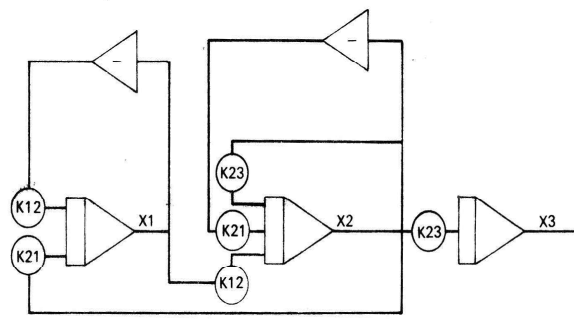
Automobile suspension:

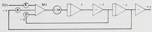
Summer: This block adds the forces acting on the system.

Scale changer: It is used to scale the input force by a factor of $M$, which is the mass of automobile. This scaling translates the force into acceleration, as according to Newton’s second law.

Integrator: The first integrator block takes the acceleration and integrates it with respect to time to give velocity, and the second integartor takes the velocity and integrate it with respect to time to give displacement.

Sign inverter: This block inverts the sign of the input signal.

The feedback loop with the integrator and sign inverter represents the effect of damping in the suspension system. A damper in a car suspension provides a force that is proportional to the velocity of the suspension’s movement but in the opposite direction, hence the inversion of the signal. The damping force is crucial for absorbing energy and preventing continuous oscillation of the car body after a disturbance (like hitting a bump).

Liver:

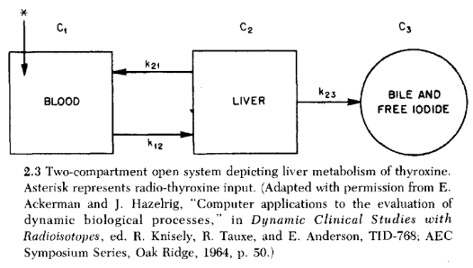
Equations: ${\dot{x}}_1=-k_{12}{x}_1+k_{21}{x}_2$ ${\dot{x}}_2=k_{12}{x}_1-(k_{21}+k_{23})x_2$ ${\dot{x}}_3=k_{23}{x}_2$

Hybrid simulation:

There are times when an analog and digital computer are combined to provide a hybrid simulation. The form taken by a hybrid simulation depends upon the application.

• One computer may be simulating the system being studied, while the other is providing a simulation of the environment in which the system is to operate. In aerospace engineering, the development and testing of new aircraft systems often involve highly sophisticated simulation setups. Here’s how a hybrid simulation might be utilized:
  • Analog Computer: Simulates the aircraft’s flight dynamics in real-time. Analog computers excel at solving differential equations that describe the aircraft’s motion, including its response to control inputs and aerodynamic forces, due to their ability to perform continuous calculations quickly.
  • Digital Computer: Models the external environment in which the aircraft operates. This includes simulating complex scenarios like weather conditions (wind, turbulence), geographical landscapes, and air traffic control systems. Digital computers are suited for these tasks because of their ability to handle large datasets, discrete events, and complex logic.
• It is also possible that the system being simulated is an interconnection of continuous and discrete subsystems, which can best be modeled by an analog and digital computer being linked together. Consider a chemical manufacturing process that involves both continuous fluid dynamics (e.g., flow, mixing, and chemical reactions in reactors) and discrete process control elements (e.g., on/off valves, switches, and digital monitoring systems).
  • Analog Computer: Used to simulate the continuous aspects of the chemical processes. Analog computing can efficiently model the nonlinear differential equations governing the fluid dynamics and chemical reactions in real-time, providing an ongoing simulation of the process behavior.
  • Digital Computer: Handles the discrete control logic and decision-making processes. It simulates the digital control system that monitors process variables (like temperature, pressure, and flow rates) and makes decisions based on predefined logic to adjust the process conditions, such as opening or closing valves and starting or stopping pumps.

The introduction of hybrid simulation required certain technological advancements for its exploitation. High-speed converters are needed to transform signals from one form of representation to another.

Discrete simulation:

Random numbers are numbers generated in a way that they are not predictable, typically deriving from physical processes, such as radioactive decay or atmospheric noise, which are inherently random. These numbers are truly random because their generation does not follow a deterministic process and cannot be reproduced given the same initial conditions.

Pseudo-random numbers, on the other hand, are generated using mathematical algorithms or deterministic processes. While they appear to be random and can pass various statistical tests for randomness, they are not truly random because if you know the algorithm and its initial state (seed), you can reproduce the entire sequence of numbers. Pseudo-random number generators (PRNGs) are widely used in computing for applications where true randomness is not strictly necessary, offering the advantage of reproducibility for debugging and analysis purposes.

A sequence of random numbers $R_1,R_2,\dots$ has two important statistical properties:

1. Uniformity: uniformly distributed across a specified range. Test for the uniformity of random numbers: If the interval between $0$ and $1$ is divided into $n$ equal intervals and total of $m$ (where $m>n$) random numbers are generated between $0$ and $1$, then the test for uniformity is that in each of $n$ intervals, approximately $\frac{m}{n}$ random numbers will fall.

2. Independence: numbers should be independent of each other; value of one number should not influence the value of the next number. Example: - auto-correlation between numbers - numbers successively higher or lower than adjacent numbers

(others, not really of numbers but of process:)

3. Reproducible (for PRNGs): given the same initial seed, a pseudo-random number generator should produce the exact same sequence of numbers

4. Periodicity: PRNGs have a finite period after which the sequence of number repeats. A good PRNG has a very long period

5. Efficiency: should generate numbers quickly and with minimal computational resources

Each random number is an independent sample drawn from a continuous uniform distribution between an interval a and b. Probability density function of this distribution is given by: $f(x)=\frac{1}{b-a},\text{ for }a\le x\le b\text{ else, }0$ Mean: $\frac{1}{2}(a+b)$

Variance: $\frac{1}{12}(b-a{)}^2$

Mid square random number generator:

This is one of the earliest method for generating the random numbers. This was used in 1950s, when the principle use of simulation was in designing thermonuclear weapons. Method is as follows:

1. Take some n digit number.
2. Square the number and select n digit number from the middle of the square number. 3. Square again this number and repeat the process.

Congruential or residual generators:

One of the common methods, used for generating the pseudo uniform random numbers is the congruence relationship: $X_{i+1}\cong (a{X}_i+c)\text{ (mod m) }i=1,2,\dots ,n$where multiplier $a$, the increment $c$ and modulus $m$ are non-negative integers. This means if $(a{X}_i+c)$ is divided by $m$, then the remainder is $X_{i+1}$. In this equation $m$ is a large number such that $m\le 2^w-1$, where $w$ is the word length of the computer in use for generating $(m-1)$ numbers and $X_0$ is seed value.

Example: Let us take, $a=3,X_0=5,c=3$ and $m=7$. Then, $4,1,6,0,3,5,4$ Thus, there are only six non-repeating numbers for $m=7$. Larger is $m$, more are the non-repeated numbers. Thus period of these set of numbers is $m$. There is a possibility that these numbers may repeat before the period $m$ is achieved. Let in the above example $m=9$, then we see that number generated are $0,3,3,3,3,\dots$.It has been shown that in order to have non-repeated period $m$, following conditions are to be satisfied:

1. $c$ is relatively prime to $m$, i.e. $c$ and $m$ have no common divisor This condition ensures that every possible number in the range $0$ to $m-1$ can be generated before the sequence repeats. Being relatively prime to $m$ means that $c$ will not introduce any additional periodicity that could cause the sequence to repeat prematurely.

2. $a\cong 1(\text{mod }g)$ for every prime factor $g$ of $m$. This ensures that the sequence will have a period that is a multiple of the prime factors of $m$. If $m$ is a composite number, this condition helps ensure that the cycle length of the LCG is maximized by making the generator cycle through all residues class modulo each of these prime factors before repeating.

Another weird one called LFSR:

An LFSR operates on a string of bits (the register) that shifts one position at each step. One or more of these bits are selected as “tap points”. The new bit that enters into the shift register is the XOR (exclusive OR) of the tap points. The choice of tap points is crucial for the quality of the pseudo-random sequence and is determined by a polynomial referred to as the feedback polynomial.

Consider a simple 4-bit LFSR with the feedback polynomial $x^4+x^3+1$. This polynomial indicates that the tap points are the 4th and 3rd bits of the register. The XOR of these bits is what gets fed back into the input of the register. Here’s how it might work, starting with an initial state (seed) of 1001:

1. Initial State: 1001. The tap points are bits 3 and 4 (from the right, starting with 1), so we XOR 1 (bit 4) and 0 (bit 3) to get 1, which is the new bit entering the register.
2. Next State: The register shifts right by 1, and the new bit (1) enters on the left: 1100.
3. Continue Process: Repeat the process of shifting and inserting the XOR of the tap points.

Testing of random numbers:

The tests can be placed in two categories, according to the properties of interest: uniformity and independence:

1. Frequency test: Use the KS or chi square test to compare the distribution of the set of numbers generated to a uniform distribution

   • The null hypothesis reads that the numbers are distributed uniformly on the interval $[0,1]$. Failure to reject means that evidence of nonuniformity has not been detected by this test. This does not imply imply that further testing of the generator for uniformity is unnecessary.

2. Autocorrelation test: Tests are correlation between numbers and compares the sample correlation to the expected correlation, zero

   • The null hypothesis reads that the numbers are distributed uniformly on interval $[0,1]$. Failure to reject the null hypothesis means that evidence of dependence has not been detected by this test. This does not imply that further testing of the generator for independence is unncessary.

Kolmogorov-Smirnov test:

is a non-parametric test of the equality of continuous one dimensional probability distribution that can be used to test whether two sample came from the same distribution.

Suppose that five numbers were generated 0.44, 0.81, 0.14, 0.05, 0.93, say with level of significance $\alpha =0.05$. First, rank the data from smallest to largest. Then compute:

$D^{+}={\text{max}}_{i\le \le N}\left\{\frac{i}{N}-R_{(i)}\right\}$

$D^{-}={\text{max}}_{i\le \le N}\left\{R_{(i)}-\frac{i-1}{N}\right\}$

$D=\text{max}(D^{+},D^{-})$

Locate the critical value, $D_{\alpha }$ for the specified significance level and the given sample size $N$. If the sample statistic $D$ is greater than the critical value, $D_{\alpha }$, the null hypothesis that the data are a sample from a uniform distribution is rejected. If $D\le D_{\alpha }$, conclude that no difference has been detected between the true distribution $\{R_1,\dots ,R_n\}$ and the uniform distribution.

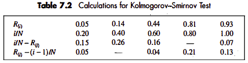
For $N\ge 40,\text{significance is }\frac{1.36}{\sqrt{N}}$

Chi-square Test:

A chi-squared test is a statistical hypothesis test in analysis of contingency tables when the sample sizes are large. In simpler terms, this test is primarily used to examine whether two categorical variables (two dimensions of the contingency table) are independent in influencing the test statistic.

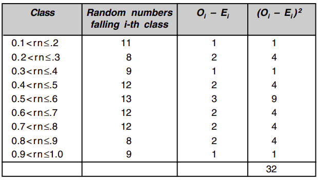
The chi-square test uses the sample statistic:

${\chi }_0^2={\sum }_{i=1}^n\frac{(O_i-E_i{)}^2}{E_i}$

It can be shown that the sampling distribution of ${\chi }^2$ is approximately the chi-square distribution with $(n-1)$ degree of freedom.

…

${\chi }^2=\frac{32}{10}=3.2$ From the ${\chi }^2$ table, we find that for degree of freedom 9, value of ${\chi }^2$ for 95% level of confidence is 16.919, which is more than our value 3.2. Thus random numbers are uniform with 95% level of confidence.

Autocorrelation test:

The following test computes the auto-correlation between every $m$ numbers ($m$ is also known as the lag), starting with the ith number. Thus, the auto-correlation ${\rho }_{im}$ between the following numbers would be of interest: $R_i,R_{i+m},\dots ,R_{i+(M+1)m}$. The value $M$ is the largest integer such that $i+(M+1)m\le N$, where $N$ is the total number of values in the sequence.

For large values of $M$, the distribution of the estimator ${\rho }_{im}$, denoted by $\widehat{{\rho }_{im}}$ is approximately normal if values are uncorrelated. Then the test statistic can be formed as follows: $Z_0=\frac{\widehat{{\rho }_{im}}}{{\sigma }_{\rho }}$ which is distributed normally with a mean of zero and a variance of 1, under the assumption of independence for large $M$.

The formula for ${\hat{\rho }}_{im}$ in a slightly different form are given by Schmidt and Taylor as follows:

${\hat{\rho }}_{im}=\frac{1}{M+1}\left[{\sum }_0^M{R}_{i+km}{R}_{i+(k+1)m}\right]-0.25$ (ex: euta sequence test garna bhanyo bhane tesko sab terms lai multiply garni, then divide by no of terms there)

and ${\sigma }_{{\rho }_{im}}=\frac{\sqrt{13M+7}}{12(M+1)}$ (and the idea goes like z-static)

Gap Test:

(upto now, the KS and chi tests were done for frequencies, now we see for gaps)

found a tutorial for KS gap test, have not found anything for chi squared? (it does not also make sense for chi)

• While frequency tests evaluate the overall distribution of values, gap tests can detect serial dependencies and patterns in the sequence not apparent from frequency analysis alone
• Gap tests asses the independence of occurrences within a sequence, which is crucial for many applications requiring random sequences
• Helps identify clustering and dispersion of specified events more effectively
• Complements frequency tests
• Useful for sparse events

Poker’s test:

This test is named after a game of cards called poker. In this game five cards are distributed to each player out of pack of fifty two cards. The cards are ranked from high to low in the following order: Ace, King, Queen, Jack, 10, 9, 8, 7, 6, 5, 4, 3, 2. Aces are always high. Aces are worth more than Kings which are worth more than Queens which are worth more than Jack, and so on. Each player is dealt five cards. The object of the game is to end up with the highest-valued hand. From best to worst, hands are ranked in the following order:

1. Royal Flush: A Royal Flush is composed of 10, Jack, Queen, King and Ace, all of the same suit.
2. Straight Flush: Compromised of five cards in numerical order, all of the same suit.
3. Four of a Kind: Four cards of the same numerical rank and another random card.
4. Full House: Of the five cards in one’s hand, three have the same numerical rank, and the two remaining card also have the same numerical rank.
5. Flush: A Flush is comprised of five cards of the same suit, regardless of their numerical rank. In a tie, whoever has the highest ranking card wins
6. Straight: Five cards in numerical order, regardless of their suits
7. Three of a Kind: Three cards of the same numerical rank, and two random cards that are not a pair.
8. Two Pair: Two sets of pairs, and another random card.
9. One Pair: One pair and three random cards.

The straight, flushes, and royals of the Poker are disregarded in the poker test.

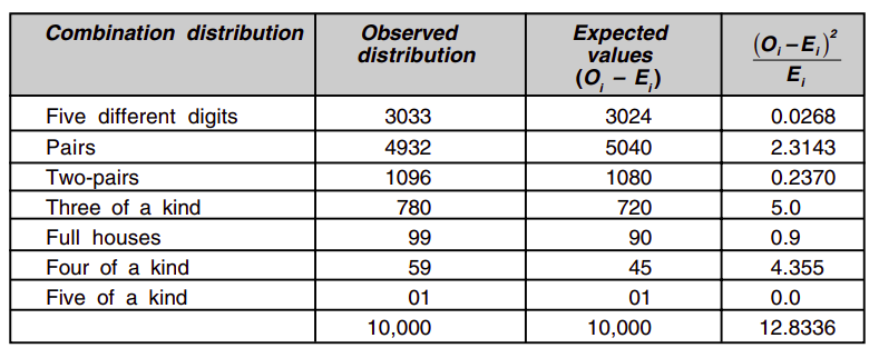
Five digit poker:

Hand Type	Probability Calculation Method	Absolute Values
1. Five different digits	C(10, 5) * 5! / 1!	30,240
2. One pair	C(10, 1) * C(9, 3) * (5! / 2!)	50,400
3. Two pairs	C(10, 2) * C(8, 1) * (5! / (2!2!))	10,800
4. Three of a kind	C(10, 1) * C(9, 2) * (5! / 3!)	7,200
5. Three of a kind + a pair	C(10, 1) * C(9, 1) * (5! / (3!2!))	900
6. Four of a kind	C(10, 1) * C(9, 1) * (5! / 4!)	450
7. Five of a kind	C(10, 1) * 5! / 5!	10

General expression: $\text{Number of ways}=C(n,r)\dots \frac{m!}{a!\times b!\times \dots }$ where,

• $C(n,r)$ is the combination representing the number of ways to choose $r$ items out of $n$ possibilities, and it can be applied multiple times as $C(n,r)\times \dots$ if the selection process is staged e.g. choosing a digit for a pair, then choosing different digits.
• $m!$ is the factorial of the total number of positions in the hand, account for all the ways to arrange the chosen digits. For poker test of five digits, $m=5$.
• $a!,b!,\dots$ represent the factorials of the counts of identical items in the hand, used to divide the total arrangements to avoid over-counting arrangements that are essentially the same due to indistinguishable digits.

Four digits:

Hand Type	Number of Ways
Four different digits	5,040
One pair + two different digits	4,320
Two pairs	270
Three of a kind + one different digit	360
Four of a kind	10

Three digits:

Hand Type	Number of Ways
Three different digits	720
One pair + one different digit	270
Three of a kind	10

Simulation of Queuing systems

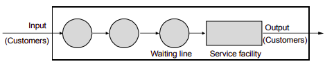
In a simple but typical queuing model, customers arrive from time to time and join a queue (waiting line), are eventually served, and finally leave the system. The term customer refers to any type of entity that can be viewed as requesting service from the system. Therefore, many service facilities, production systems, repair and maintenance facilities, communications and computer systems, and transport and material-handling systems can be viewed as queuing systems.

Waiting in queues incur cost, whether human are waiting for services or machines waiting in a machine shop. On the other hand if service counter is waiting for customers that also involves cost. In order to reduce queue length, extra service centers are to be provided but for extra service centers, cost of service becomes higher. On the other hand excessive wait time in queues is a loss of customer time and hence loss of customer to the service station.

Ideal condition in any service center is that there should not be any queue. But on the other hand service counter should also be not idle for long time. Optimization of queue length and wait time is the object theory of queuing.

The population:

The difference between finite and infinite population models is how the arrival rate is defined. In an infinite population model, the arrival rate (i.e. the average number of arrivals per unit of time) is not affected by the number of customers who have left the calling populations and joined the queuing system. When the arrival process is homogeneous over time, the arrival rate is usually assumed to be constant. On the other hand, for finite calling population, the arrival rate to the queuing system does depend on the number of customers being served and waiting.

System capacity:

There is a limit to the number of customers that may be in the waiting line or system.

The arrival process:

The arrival process for infinite population is usually characterized in terms of inter-arrival times of successive customers. Arrivals may occur at scheduled times or at random times. When at random times, the interval times are usually characterized by a probability distribution. The most important model for random arrivals is the Poisson arrival process. If $A_n$ represents the interarrival time between customer $n-1$ and customer $n$ ($A_1$ is the actual arrival time of the first customer), then, for a Poisson arrival process, $A_n$ is exponentially distributed with mean $1/\lambda$ time units. The arrival rate is $\lambda$ customers per time unit.

For finite population …

Queue behavior:

Queue discipline refers to the logical ordering of customers in a queue and determines which customer will be chosen for service when a server becomes free. Common queue disciplines include first-in-first-out (FIFO); last-in-first-out (LIFO); service in random order (SIRO); shortest processing time first (SPT); and service according to priority (PR). . Notice that a FIFO queue discipline implies that services begin in the same order as arrivals,.but that customers could leave the system in a different order because of different-length service times.

Service times and mechanism:

The service times of successive arrivals are denoted by $S_1,S_2,\dots$. They may be constant or of random duration.

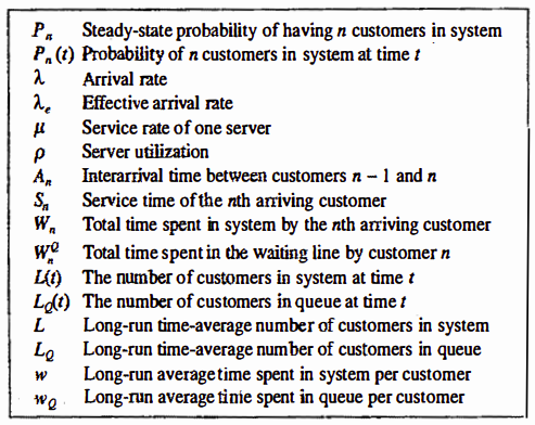
Notations:

Recognizing the diversity of queuing systems, Kendall proposed a national system for parallel server systems which has been widely adopted. An abridged version of this convention is based on format $A/B/c/q/N/K$.

• arrival pattern (distribution of intervals between arrivals)
• service pattern (distribution of service duration)
• number of servers,
• queue discipline (FIFO, LIFO). Omitted for FIFO or if not specified
• system capacity. Omitted for unlimited queues
• population size (number of possible customers). Omitted for open systems

Common symbol for A and B include:

• D (constant or deterministic)
• M (exponential or Markov)
• $E_k$ (Erlang of order k)
• $H$ (hyper-exponential)
• $G$ (arbitrary or general)

Additional notation:

Conservation law:

The average number of customers in the system at an arbitrary point in time is equal to the average number of arrivals per unit time, times the average time spent in the system. $L=\lambda w$

Server utilization in D/D/1 ($\lambda$ and $\mu$ given) The percentage of time during which the server is busy processing jobs during a simulation.

In a single server queue, the average number of customers being served at an arbitrary point in time is equal to server utilization. $\rho =L=\lambda w$. For the server subsystem, the average system time is $w=\frac{1}{\mu }$ . Hence, $\rho =\frac{\lambda }{\mu }$ that is,. the long-run server utilization in a single-server queue is equal to the average arrival rate divided by the average service rate. For a single-server queue to be stable, the arrival rate $\lambda$ must be less than the service rate $\rho$:

Server utilization in D/D/c ($\lambda$ and $\mu$ given)

$\rho =\frac{\lambda }{c\mu }$

By varying $\lambda$ and $\mu$. server utilization can assume any value between 0 and 1, yet there is never any line whatsoever. What, then, causes lines to build, if not a high server utilization? In general, it is the variability of interarrival and service times that causes lines to fluctuate in length.

Steady state of infinite population M/M/1:

(with some calculations and conservation applies)

The average number of customers at time $t$, in the system is $L_S=\frac{\lambda }{\mu -\lambda }=\frac{\rho }{1-\rho }$

Probability of $n$ customers being in the system can also be expressed as $P_n={\rho }^n(1-\rho )$

The average number of customers in the queue (not being served) $L_Q=L_S-\rho =\frac{{\lambda }^2}{\mu (\mu -\lambda )}=\frac{{\rho }^2}{1-\rho }$

(samjhina ko lagi remember $w=\frac{1}{\mu -\lambda }$ when previously it was just $\frac{1}{\mu }$)

Also, steady probability of having customers in system: $P_n=(1-\rho ){\rho }^n$

Markov Chains

A Markov process is a stochastic model describing a sequence of possible vents in which the probability of each event depends only on the state attained in the previous event. The changes of states of the system are called transitions. The probabilities associated with various state changes are called transition probabilities. he process is characterized by a state space, a transition matrix describing the probabilities of particular transitions, and an initial state (or initial distribution) across the state space. By convention, we assume all possible states and transitions have been included in the definition of the process, so there is always a next state, and the process does not terminate.

If the state space if finite, the transition probability distribution can be represented by a matrix, called the transition matrix, with the $(i,j)$th element of $P$ equal to: $p_{ij}=Pr(X_{n+1}=j|X_n=i)$ Since each row of $P$ sums to one and all elements are non-negative, $P$ is a right stochastic matrix.

Time homogeneous Markov chain:

If the MC is time homogeneous, then the transition matrix $P$ is the same after each step, so the k-step transition probability can be computed as the k-th power of the transition matrix, $P^k$. If the Markov chain is irreducible and aperiodic, then there is a unique stationary distribution $\pi$.

Verification and validation

The engineers and analysts who use the model outputs to aid in making design recommendations and the managers who make decisions based on these recommendations - justifiably look upon a model with some degree of skepticism about its validity.

The goal of the validation process is two fold:

1. to produce a model that represents true system behavior closely enough for the model to be used as a substitute for the actual system for the purpose of experimenting with the system, analyzing system behavior, and predicting system performance; and
2. to increase to an acceptable level the credibility of the model, so that the model will be used by managers and other decision makers

Validation should not be seen as an isolated set of procedures that follows model development, but rather as an integral part of model development. Conceptually, however, the verification and validation process consists of the following components:

1. Verification is concerned with building the model correctly. It proceeds by the comparison of the conceptual model to the computer representation that implements that conception. It asks the questions:

   • Is the model implemented correctly in simulation software?
   • Are the input parameters and logical structure of the model represented correctly?

2. Validation is concerned with building the correct model. It attempts to confirm that a model is an accurate representation of the real system. Validation is usually achieved through the calibration of the model, an iterative process of comparing the model to actual system behavior and using the discrepancies between the two, and the insights gained, to improve the model. This process is repeated until the model accuracy is judged to be acceptable.

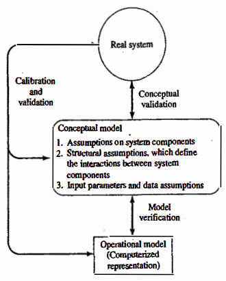
Model building, verification and validation:

Observation and Consultation: Gather system behavior data and consult experts for in-depth knowledge.

Conceptual Model Creation: Develop a model with assumptions about the system’s structure and inputs, then validate against the real system.

Operational Model Implementation: Use simulation software to build the model, iteratively refining through comparison and validation with the real system.

Verification

The purpose of model verification is to assure that the conceptual model is reflected accurately in the operational model.

Most common sense suggestions:

• Have the operational model checked by someone other than its developer, preferably an expert in simulation software
• Make a flow diagram that includes each logically possible action a system can take when an event occurs, and follow the model logic for each action for each event type
• Closely examine the model output for reasonableness under a variety of settings of the input parameters
• Make the operational model as self-documenting as possible.
• The Interactive Run Controller (IRC) or debugger is an essential component of successful simulation model building. Even the best of simulation analysts makes mistakes or commits Iogical errors when building a model.
• Graphical interfaces are recommended for accomplishing verification and validation. The graphical representation of the model is essentially a form of self-documentation.

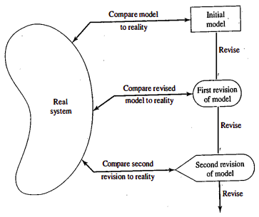
Calibration and validation of models

Validation is the overall process of comparing the model and its behavior to the real system and its behavior. Calibration is the iterative process of comparing the model to the real system, making adjustments (or even major changes) to the model, comparing the revised model to reality, making additional adjustments, comparing again, and so on. The comparison of the model to reality is carried out by a variety of tests-some subjective, others objective.

• Subjective tests usually involve people, who are knowledgeable about one or more aspects of the system, making judgments about the model and its output.
• Objective tests always require data on the system’s behavior, plus the corresponding data produced by the model. Then one or more statistical tests are performed to compare some aspect of the system data set with the same aspect of the model data set

As an aid in the validation process, Naylor and Finger formulated three step approach that has been widely followed:

1. Build the model that has high face validity
2. Validate model assumptions
3. Compare the model input-output transformations to corresponding input-output transformations for the real system.

Face validity:

The first goal of the simulation modeler is to construct a model that appears reasonable on its face to model users and others who are knowledgeable about the real system being simulated.

Involve credible users: can aid in identifying model deficiencies, to ensure realism is built into model through reasonable assumption regarding system structure and through reliable data.

Conduct sensitivity analysis: model user is asked whether the model behaves in expected way when one or more input variables are changed. For ex: in most queuing systems, if the arrival rate of customers were to increase, it would be expected that utilization of servers, lengths of lines, and delays tend to increase.

Validation of model assumptions:

Structural assumptions

• defn: concerns how the system operates, involving simplifications and abstractions of reality to model the system structure
• ex: in a bank, structural assumption include the arrangement of customer queues, whether the number of tellers is fixed or variables, and policies of customer changing lines
• validation: these assumptions are verified through direct observations and discussions with individuals familiar with the system, such as managers and tellers

Data assumptions

• defn: based on collection reliable data and conducting correct statistical analyses on the data
• ex: for a bank, data might be gathered on the inter-arrival times of customers during peak and slack periods, as well as service times for different types of accounts.
• validation: reliability is further assured by using objective statistical tests to check for data homogeneity and tests for correlations to confirm the randomness of the sample, and validation the statistical model using goodness of fit\

Validating input-output transformations:

The ultimate test of a model is the model’s ability to predict the future behavior in the real system when the model input data match the real inputs and when a policy implemented in the model is implemented at some point in the system. Furthermore, if the level of some input variables were to increase or decrease, the model should accurately predict what would happen in the real system under similar circumstances.

In this phase of the validation process, the model is viewed as an input-output transformation - that is, the model accepts values of the input parameters and transforms these inputs into output measures of performance.

Using historical input data:

• Instead of validating the model input-output transformations by predicting the future, the modeler could use historical data that have been reserved for validation purposes only - that is, if one data set has been used to develop and calibrate model, it is recommended that a separate data set be used as the final validation set.

Turing test:

• The Turing test involves mixing real performance reports with simulated reports and asking experts to identify which ones are simulated. If experts can’t reliably distinguish between real and fake, it suggests the model closely mimics reality, indicating a successful simulation. This method, useful when statistical tests are inadequate, helps refine the model based on expert feedback, enhancing its credibility.

Output analysis

Once a stochastic variable has been introduced into a simulation model, almost all the system variables describing the system’s behavior also become stochastic, because of the way endogenous events make one variable depend upon another. The values of most, if not all, of the system variables will fluctuate as the simulation proceeds, so that no one measurement can be arbitrarily taken to represent the value of a variable.

Usually, a random variable is drawn from an infinite population that has a stationary probability distribution with a finite mean, $\mu$ and finite variance, ${\sigma }^2$. This means that the population distribution is not affected by the number of samples already made, nor does it change with time. Random variables that meet all these conditions are said to be iid. Under broad conditions that can be expected to hold for simulation data, the central limit theorem can be applied to iid data. The theorem sates that the sum of iid variables, drawn from a population that that mean $\mu$ and variance of ${\sigma }^2$ is approximately distributed as a normal variable with mean $n\mu$ and variance of $n{\sigma }^2$. Any normal distribution can be transformed into a standard normal distribution that has a mean of $0$ and a variance of $1$. Let $x_i(i=1,2,\dots ,n)$ be the $n$ iid random variables. Using the central limit theorem, and applying transformation: $z=\frac{\bar{x}-\mu }{\frac{\sigma }{\sqrt{n}}}$The variable $\bar{x}$ is the sample mean. It can be shown to be consistent estimator for the mean of the population from which the sample is drawn.

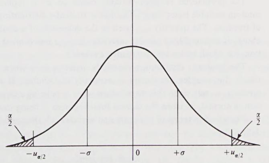
The integral from $-\infty$ to a value $u$ is the probability that $z$ is less than or equal to $u$. Suppose that value of $u$ is chosen so that integral is $1-\alpha /2$, where $\alpha$ is some constant less than $1$, and denote this value by $u_{\alpha /2}$. The probability that $z$ is greater than $u_{\alpha /2}$ is then $\alpha /2$. Consequently, the probability that $z$ lies between $-u_{\alpha /2}$ and $u_{\alpha /2}$ is $1-\alpha$. That is, $Pr\{-u_{\alpha /2}\le z\le u_{\alpha /2}\}=1-\alpha$ In terms of the sample mean, this probability statement can be written: $Pr\{\bar{x}+\frac{\sigma }{\sqrt{n}}{u}_{\alpha /2}\ge \mu \ge \bar{x}-\frac{\sigma }{\sqrt{n}}{u}_{\alpha /2}\}=1-\alpha$ The constant $1-\alpha$ is the confidence level and the interval. Typically confidence level might be 90% in which case $u_{\alpha /2}$ is 1.65. The statement then says that $\mu$ will be covered by the confidence interval $\bar{x}\pm 1.65\sigma /\sqrt{n}$ with probability 0.9; meaning that, if the experiment is repeated many times, the confidence interval can be expected to cover the value $\mu$ on 90% of the repetitions.

In practice, the population variance ${\sigma }^2$ is not usually known; in which case, it is replaced by an estimate calculated from the formula:

$s^2=\frac{1}{n-1}{\sum }_{i=1}^n(x_i-\bar{x}{)}^2$ The normalized random variable based on ${\sigma }^2$ is replaced by a normalized random variable based on $s^2$. This has a Student-t distribution, with $n-1$ degrees of freedom. The quantity $u_{\alpha /2}$ used in the definition of a confidence interval given above, is replaced by a similar quantity, $t_{n-1,\alpha /2}$, based on the Student-t distribution, for which tables are also readily available.

Simulation run statistics:

It was assumed that the observations are mutually independent, and it is assumed that the distribution from which they are drawn is stationary. Unfortunately, many statistics of interest in a simulation do not meet these conditions. To illustrate the problems that arise in measuring statistics from simulation runs, a specific example will be discussed.

Consider a single-server system in which the arrivals occur with a Poisson distribution and the service time has an exponential distribution. Suppose the study objective is to measure the mean waiting time, defined as the time entities spend waiting to receive service and excluding the service time itself. In a simulation run, the simplest approach is to estimate the mean waiting time by accumulating the waiting time of $n$ successive entities and dividing by $n$. This measure, the sample mean, is denoted by $\bar{x}(n)$ to emphasize the fact that its value depends upon the number of observations taken.

… (formula here) …

Waiting times measured this way are not independent. Whenever a waiting line forms, the waiting time of each entity on the line clearly depends upon the waiting time of its predecessors. Any series of data that has this property of having one value affect other values is said to be autocorrelated.

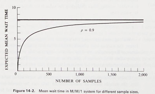
Another problem that must be faced is that the distributions may not be stationary. In particular, a simulation run is started with the system in some initial state, frequently the idle state, in which no service is being given and no entities are waiting. The early arrivals then have a more than normal probability of obtaining service quickly, so a sample mean that includes the early arrivals will be biased. As the length of the simulation run is extended, and the sample size increases, the effect of the bias will die out.

Replication of runs:

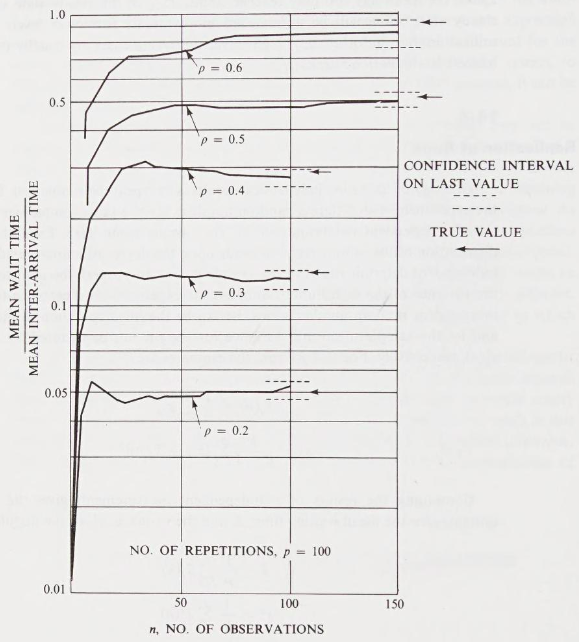
One way of obtaining independent results is to repeat the simulation. Repeating the experiment with different random numbers for the sample size $n$ gives a set of independent determinations of the sample mean $\bar{x}(n)$. Even though the distribution of the sample mean depends upon the degree of auto-correlation, these independent determinations of the sample mean can properly be used to estimate the variance of the distribution. Suppose the experiment is repeated $p$ times with independent random number series. Let $x_{ij}$ be the $i$th observation in the $j$th run, and let the sample mean and variance for the $j$th run be denoted by ${\bar{x}}_j(n)$ and $s_j^2(n)$, respectively. For that $j$th run, the estimates are: ${\bar{x}}_j(n)=\frac{1}{n}{\sum }_{i=1}^n{x}_{ij}$

$s_j^2=\frac{1}{n-1}{\sum }_{i=1}^n[x_{ij}-{\bar{x}}_j(n){]}^2$

Combining the results of $p$ independent measurements give the following estimates for the mean waiting time, $\bar{x}$ and the variance $s^2$, of the population: $\bar{x}=\frac{1}{p}{\sum }_{j=1}^p{\bar{x}}_j(n)$ $s^2=\frac{1}{p}{\sum }_{j=1}^p{\bar{s}}_j^2(n)$ Results are shown for server utilization $0.1,0.3,0.4,0.5,$ and $0.6$. In each case, the experiment has been repeated from an initial idle state, different random numbers being used on each repetition.

The $p$ repetitions of $n$ observations involve a total of $N=pn$ observations. In a computer based simulation, the total time spent carrying out calculations will be roughly proportional to $N$. The question of how best to divide the $N$ observations between the number of repetitions and the length of the individual runs.

Take N = 12,800

• $n=2560,p=5$: where 83% of the confidence interval covered the true mean.
• $n=320,p=40$: dropped to 9%

Elimination of initial bias:

The experiments above show the need to remove the initial bias, or reduce its effect. Two general approaches can be taken to remove the bias:

• the system can be started in more representative state than the empty state,
• or the first part of the simulation run can be ignored

(read the another book part)

(from another book:)

Output analysis is the examination of data generated by a simulation. Its purpose is either to predict the performance of a system or to compare the performance of two or more alternative system designs. Consider one run of a simulation model over a period of time $[0,T_E]$. Since the model is an input-output transformation, and since some of the model input variables are random variables, it follows that the model output variables are random variables. Consider the estimation of a performance parameter, $\theta$, of a simulated system. It is desired to have a point estimate and an interval estimate. The length of the interval estimate is a measure of the error in the point estimate. The simulation output data are of the form $\{Y_1,Y_2,\dots ,Y_n\}$ for estimating $\theta$; we refer to such output data as discrete time data.

Point estimation:

The point estimator of $\theta$ based on the data $\{Y_1,\dots ,Y_n\}$ is defined by: $\hat{\theta }=\frac{1}{n}{\sum }_{i=1}^n{Y}_i$ where $\hat{\theta }$ is a sample mean based on a sample of size $n$. The point estimator $\hat{\theta }$ is said to be unbiased for $\theta$ if its expected value is $\theta$ - that is, if $E(\hat{\theta })=\theta$ In general, however, $E(\hat{\theta })\ne \theta$ and $E(\hat{\theta })-\theta$ is called the bias in the point estimator $\theta$. It is desirable to have estimators that are unbiased, or, if this is not possible, have a small bias relative to the magnitude of $\theta$.

Confidence-interval estimation:

Suppose that model is an normal distribution with mean $\theta$ and variance ${\sigma }^2$, both unknown. To make the example concrete, let ${\bar{Y}}_i$ be the average cycle time for parts produced on the $i$th replication (representing a day of production) of simulation. Therefore, $\theta$ is the mathematical expectation of $\bar{Y}$, and $\sigma$ represents the day-to-day variation of the average cycle time. Suppose our goal is to estimate $\theta$. The natural estimator is overall mean of independent replications, but $\bar{Y}$ is not $\theta$, it is an estimate, based on the sample, and it has error. A confidence interval is a measure of that error. Let, $S^2=\frac{1}{R-1}{\sum }_{i=1}^R(Y_i-\bar{Y}{)}^2$be the sample variance across the $R$ replications. The usual confidence interval, which assumes the $Y_i$ are normally distributed, is $\bar{Y}\pm t_{\alpha /2,R-1}\frac{S}{\sqrt{R}}$where $t_{\alpha /2,R-1}$ is the quartile range of the $t$ distribution with R-1 degrees of freedom that cuts off $\alpha /2$ area of the each tail.

initialization bias:

There are several methods of reducing the point-estimator bias caused by using artificial and unrealistic initial conditions in a steady-state simulation.

The first method is to initialize the simulation in a state that is more representative of long-run conditions. This method is sometimes called intelligence initialization. Example include placing customers in queue and in service in a queuing simulation. There are at least two ways to specify the initial conditions intelligently.

• If the system exists, collect data on it and use these data to specify more nearly typical conditions. This method sometimes requires a large data collection effort. If the system being modeled does not exist, if it is a variant of an existing system - this method is impossible to implement.
• A related idea is to obtain initial conditions from a second model of the system that has been simplified enough to make it mathematically solvable. The simplified model can be solved to find long-run expected or most likely conditions - such as the expected number of customer sin the queue - and these conditions can be used to initialize the simulation.

A second method is reduce the impact of initial conditions, possibly used in conjunction with the first, is to divide each simulation run into two phases: first, an initialization phase, from time $0$ to time $T_0$, followed by a data-collection phase from time $T_0$ to the stopping time $T_0+T_E$ - that is, simulation begins at time $0$ under special initial conditions $I_0$ and runs for a specified period of time $T_0$. Data collection on the response variables of interest does not being until time $T_0$, denoted by $I$, should be more nearly representative of steady-state behavior than are the original initial conditions at time $0$, $I_0$. In addition, the length $T_E$ of the data-collection phase should be long enough to guarantee sufficiently precise estimates of steady-state behavior.

(example about bias in averages, so deleting idea)

Ensemble averages can be smoothed further by plotting a moving average, rather than the original ensemble averages. In a moving average, each plotted point is actually the average of several adjacent ensemble averages. (…)

Simulation Software

There are many features that are relevant when selecting simulation software. We offer the following advice when evaluating and selecting simulation software:

• Do not focus on a single issue, such as ease of use. Consider the accuracy and level of detail obtainable, ease of learning, vendor support, and applicability to your applications.
• Execution speed is important
• Beware of advertising claims and demonstrations.
• (some others)

JAVA:

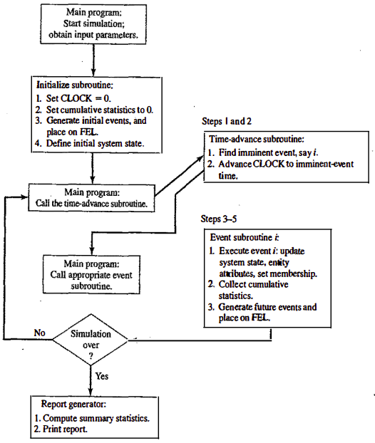
Java is a widely used programming language that bas been used extensively ib simulation. It does not, however, provide any facilities directly aimed at aiding the simulation analyst, who therefore must program all details of the event-scheduling/time-advance algorithm, the statistics-gathering capability, the generation of samples from specified probability distributions, and the report generator. However, the runtime library does provide a random-number generator. Unlike with FORTRAN or C, the object-orientedness of Java does support modular construction of large models.

The following components are common to almost all models written in Java:

• Clock: a variable defining simulated time;
• Initialization method: a method to define the system time at time 0
• Min-time event method: a method that identifies the imminent event, that is, the element of the future event list that has the smallest time-stamp
• Event methods: a method to update system state (and cumulative statistics) when that event occurs
• Random-variate generators: methods to generate samples from desired probability distributions
• Main program: to maintain overall control of the event-scheduling algorithm
• Report generator: a method that compute summary statistic from cumulative statistics and prints report at the end of the simulation

Single server queue simulation in Java: (not for me man)

GPSS:

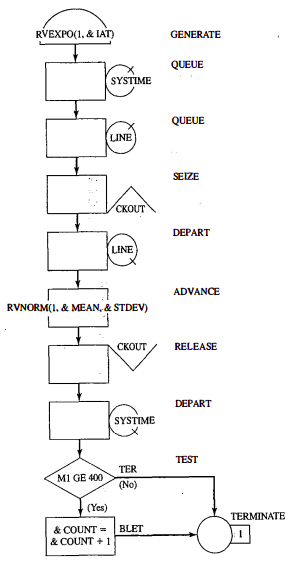
GPSS is a highly structured, special-purpose simulation programming language based on the process-interaction approach and oriented towards queuing systems. (This approach contrasts with event scheduling or activity scanning methods). A block diagram provides a convenient way to describe the system being simulated. There are over 40 standard blocks in GPSS. Entities called transactions may be viewed as flowing through the block diagram. Blocks represent events, delays, and other actions that affect transaction flow. Thus, GPSS can be used to model any situation where transactions (entities, customers, units of traffic) are flowing through a system (e.g. network of queues, with the queues preceding scarce resources). The block diagram is converted to block statements, control statements are added, and the result is a GPSS model.

The first version of GPSS was released by IBM in 1961. It was first process-interaction simulation langugae and became popular; it has been implemented a new and improved by many parties since 1961, with GPSS/H being the most widely used version in use today.

Blocks:

• The GENERATE block represents the arrival event, with the inter-arrival times specified by RVEXPO(1, &IAT)

  • RVEXPO stands for random variable, exponentially distributed
  • 1 indicates the random-number stream to use
  • &IAT indicates that the mean time for exponential distribution comes from a so called ampervarable

• The next block is QUEUE with a queue named SYSTIME. It should be noted that the QUEUE block is not needed for queues or waiting lines to form in GPSS. The true purpose of the QUEUE block is to work in conjunction with the DEPART block to collect data on queues or any other subsystems. Here, we want to measure the system response time - that is, the time a transaction spends in the system. Placing a QUEUE block at the point that transaction enter the system and placing the counterpart of the QUEUE block, the DEPART block, at the point that the transactions complete their processing causes the response times to be collected automatically. The purpose of DEPART is to signal the end of data collection for an individual transaction. The QUEUE block (with name LINE) begins data collection for the waiting line before the cashier.

• The customers may or may not have to wait for the cashier. Upon arrival to an idle checkout counter, or after advancing to the head of the waiting line, a customer captures the cashier, as represented by the SEIZE block with the resource named CHECKOUT, once the transaction representing a customer captures the cashier represented by the resource CHECKOUT, the data collection for the waiting-line statistic ends.

• The transaction’s service time at the cashier is represented by an ADVANCE block

  • RVNORM indicates random variable, normally distributed
  • 1 for stream
  • others variables

• Next, the customer gives up the use of the facility CHECKOUT with a RELEASE block. The end of the data collection for response times indicated by the DEPART block for the queue SYSTIME.

• Next, there is a TEST block that checks to see whether the time in the system, M1, is greater than or equal to 4 minutes.

SSF: (poor guy)

Simulation of computer systems

Computer system are incredibly complex. A computer system exhibits complicated behavior at time scales from the time to flip a transistor’s state (on the order of $10^{-11}$ seconds) to the time it takes a human to interact with it. Computer systems are designed hierarchically, in an effort to manage the complexity.

• A high level of abstraction (system level), one might view computational activity in terms of tasks circulating among servers, queuing for service when a server is busy.
• A lower level in the hierarchy can view the activity as being among components of a given processor (its registers, its memory hierarchy).
• At a lower level still, one views the activity of functional units that make up central processing unit, and,
• at an even lower level, one can view the logical circuitry that makes it all happen.

(pic)

Simulation is used extensively at every level of this hierarchy, with some results from one level being used at another. For instance, engineers working on designing a new chip will begin by partitioning the chip functionally (e.g the subsystem that does arithmetic, the subsystem that interacts with memory and so on), establish interfaces between the subsystems, then design and test the subsystems individually.

• Given a subsystem design, the electrical properties of the circuit are first studied by using a circuit simulator that solves differential equations describing electrical behavior. At this level, engineers work to ensure the correctness of signals’ timing throughout the circuit.
• Once this level of validation has been achieved, the electrical behavior is abstracted into logical behavior (e.g. signals formerly though of as waveforms are now thought as logical 1’s and 0’s). A different type of simulator is next used to test correctness of logical inputs.
• Once a chip’s subsystems are designed an tested, the designs are integrated, and then the whole subsystem is subjected to testing, again by simulation.
• At a higher level, one simulates by using functional abstractions. For instance, a memory chip could be modeled simply as an array of numbers, and a reference to memory as just an indexing operation. A special type of description language exists for this level, called register-transfer-language.
• At a higher level still, one might study how an Input-Output (I/0) system behaves in response to execution of a computer program. The program’s behavior may be abstracted to the point of being modeled, but with some detailed description of I/0 demands (e.g., with a Markov chain that with_ some specificity describes an I/0 operation as the Markov chain transitions).

Different levels of abstraction serve to answer different sorts of questions about a computer system, and different simulation tools exist for each level. Highly abstract models rely on stochastically modeled behavior to estimate high-level system performance, such as throughput (average number of ‘jobs” processed per unit time) and mean response time (per job). Such models can also incorporate system failure and repair and can estimate metrics such as mean time to failure and availability. Less abstract models are used to evaluate specific systems components. A study of an advanced CPU design might be aimed at estimating the throughput (instructions executed per unit time); a study of a hierarchical memory system might seek to estimate the fraction of time that a sought memory reference was found immediately in the examined memory.

Simulation tools:

• Circuit simulations
• VHDL
• RTL

High level computer system simulation:

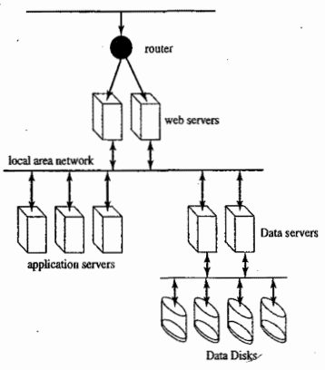
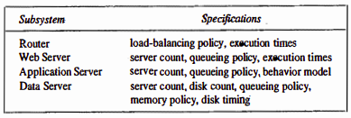
A computer that provides a major website for searching and links to sites for travel, commerce, entertainment, and the like wishes to conduct a capacity-planning study. The overall architecture of its system is:

• At the back end, one finds data servers responsible for all aspects of handling specific queries and updating database

• Data servers receive requests for service from application servers - machines dedicated to running specific applications (e.g. a search engine) supported by the site.

• In front of the applications are Web servers, which manage the interaction of applications with the WWW

• The portal to the whole system is a load balancing router that distributes requests directed to the website among the Web servers. All entries into the system are through a dedicated router, which examines the request and forwards it to some Web server.

The goal of the study is to evaluate the site’s ability to handle load at peak periods. The desired output is an empirical distribution of the access response time. Thus, the high-level simulation should focus on the impact of timing at each level that is used, system factors that affect that timing, and the effects of timing on contention for resources. To understand where those delays occur, let us consider the processing associated with a typical query.

A Web server can be though of as having

• one queue of threads of new requests,
• a second queue of threads that are suspended awaiting a response from an application server,
• and a third queue of threads ready to process responses from application servers An accepted request from the router creates a new request thread.

An application request is modeled as a sequence of sets of request from data servers, interspersed with computational bursts for example,

• burst 1: request data from D1, D3, and D5
• burst 2: request data from D1 and D2
• burst 3: …

In this model, we assumed that all data requests from a set must be satisfied before the subsequent computational burst can begin. Query search on a database is an example of an application that could generate a long sequence of bursts and data requests, with large numbers of data requests in each set.

For each application, we will maintain a list of threads that are ready to execute and a list of threads that are suspended awaiting responses from data servers.

Requires specification of Web system model:

The query-response-time distribution can be estimated by measuring, for each query, the time between at which a request first hits the router and the time at which the Web-server thread communicates the results. From the set of simulated queries, one can build up a histogram.

CPU simulation:

Next consider a lower level abstraction of simulation of CPU. Whereas the high level simulation of the previous example treated execution time of a program as a constant, at the lower level we do the simulation to discover what the execution time is.The input driving this simulation is a stream of instructions. The simulation works through the mechanics of CPU’s logical design to find out what happens in response to that stream, how long it takes to execute the program, and where bottlenecks exist in the CPU design.

The main challenge to making effective use of a CPU is to avoid stalling it; stalling happens whenever the CPU commits to executing an instruction whose inputs are not all present. A leading cause of stalls is the latency delay between CPU and the main memory, which can be tens of CPU cycles. One instruction might initiate a read - for example, \text{load }$2, 4($3) which is an assembly language statement that instructs the CPU to use the data in register 3 (after adding value 4 to it) as an memory address to put the data into register 2. If the CPU insisted on waiting for that data to appear in register 2 before further execution, the instruction could stall the CPU for a long time if the referenced address is not found in the cache. High-performance CPUs avoid this by recognizing that additional instructions can be executed, up to the point where the CPU attempts to execute an instruction that reads the contents of register 2.

Modern microprocessors add some additional capabilities to exploit instruction level parallelism. The technique of pipeline has long been recognized as a way of accelerating the execution of computer instructions. Pipelining exploits the fact that each instruction goes sequentially through several stages in the course of being processed; separate hardware resources are dedicated to each stage, permitting multiple instructions to be in various stages of processing concurrently.

Typical stages of ILP CPU cycle:

1. Instruction fetch: from memory
2. Instruction decode: what operation and what registers
3. Instruction issue: issue when no constraints, may be unavailability of registers or functional unit
4. Instruction execute: perform:
5. Instruction complete: store data in registers
6. Instruction graduate: graduate instructions in order they appear in stream

Ordinary pipelines permit at most one instruction to be represented in each stage; the degree of parallelism (number of concurrent instructions) is limited to the number of stages. This necessarily implies the possibility of executing some stages of successively fetched instructions out of order. For example, it is entirely possible for the $n$th instruction, $I_n$, to be constrained from being executed for several clock cycles while the next instruction, $I_{n+1}$ is not so constrained. An ILP processor will push the evaluation of $I_{n+1}$ along as far as it can without waiting on $I_n$. However, the instruction raudate stages will impose order and insist on graduating $I_n$ before $I_{n+1}$.

(random example goes here)

Memory simulation:

(not doing this, wish me luck)