Signals Fundaments

What is signal

SIGNALS: In signal processing, a signal is a function that conveys information about a phenomenon. Any quantity that can vary over space or time can be used as a signal to share messages between observers 1. Analog signal: -Is a continuous wave representing some quality (usually electrical) that varies over time. -Represented by sine waves -$<Features>$ 2. Digital signal: -A discrete waves that carries information in binary form -Represented by square waves -$<Features>$

COMMUNICATION: >A collection of individual components capable of interconnection and interoperation to faciliate transfer of data between a source and a receiver via from of transmission media. >Types: -A simplex communication sends information in one direction only. Eg: TV and radio broadcasting -A duplex communication system is a system composed of two connected parties or devices which can communicate wih one another in both directions. In full-duplex system, both parties can communicate with each other simultaneously. Example of a full-duplex is plain old telephone service. In half-duplex, both parties can communicate with each other, but not simultaneously; the communication is one direction at a time. An example of a half-duplex device is a walkie-takie.

>Key components:
	-Sources: Sources can be classified as electric or non-electric; they are the origins of a message or input signal. Examples of sources include:
		Audo files, GIFs, Email messages, Human voice, Electromagnetic radiation

	-Input transducers: Sensors, like microphones and cameras, capture non-electric sources, like sound and light (respectively), and convert them into electrical signals. These types of sensors are called input transducers in modern analog and digital communication systems. Without input transducers there would not be an effective way to transport non-electric sources or signals over great distances
		Microphones, Camera, Keyboards, Mouse, Accelerometers

	-Transmitter: Once the source has been converted into an electric signal, the transmitter will modify this signal for efficient transmission. In other to do this, the signal must pass through an electronic circuit containing the following components:
		Noise filter, ADC, Encoder, Modulator, Signal amplifier

	-Communication channel: Refers to the medium by which a signal travels. Two types of medias by which electric signals travel, i.e. guided and unguided. Guided media refers to any medium that can be directed from transmitter to receiver by means of connecting cables. The other type of media, unguided media, refers to any communication channel that creates space between the transmitter and receiver

	-Receiver: The goal of the receiver is to capture and reconstruct the signal before it passed through the transmitter
		Noise filter, DAC, Decoder, Demodulator, Signal amplifier

	-Output transducer: The output transducer simply converts the electric signal (created by the input transducer) back into its original form
		Speakers, Monitors, Motors, LEDs

CLASSIFICATION OF CONTINOUS SIGNALS: (Examples, Figures, What implication they have on their spectrum?) 1. Reguarity: >Determinisitc signals are precisely determined at an arbitrary time instant; their simulation implies searching for proper analytic function to describe them explicity or with highest accuracy. A determinisitc signal has no uncertaintly with respect to its value at any instant of time. >Random singals cannot be described analytically at an arbitrary time instant owing to its stochastic nature; such signals cannot be desribed in deterministic functions or by their assemblage and are subject to the probability theory and mathematical statisstics.

	-Recognition of signals as deterministic and random is conditional in a sense. There are not deterministic physical processes at all, at least because of noise that exists everywhere. The question is, however, how large is this noise? If it is negligible, as compared to the signal value, then the signal is assumed to be deterministic. If not, the signal is random, and stochastic methods would be in order for its description.

2. Periodicity:
	>Periodic signals reiterate through values through the equal time duration T called a period of repetition. For such signals the following holds true:
			x(t) = x(t \pm nT)
	where, x(t) is a signal and n = 0,1,2,...It seems obvious that simulation implies that a signa may be described only on the time interval T and then repeated n times with period T.

	>Single signals or nonperiodic signals do not exhibit repitions on the unlimited time interva and therefore the equality cannot be applied
		
	-When a continuous time signal is a mixture of two periodic signals with fundamental time periods T1 and T2, then the continuous time signals will be periodic, if the ratio of T1 and T2 (ie T1/T2) is a rational number. Now the periodicity of the continuous time signal will be the LCM of T1 and T2.

3. Symmetricity:
	>Even signals exhibits symmetry with respect to t=0 such that they satistify the condition,
			x(-t) = x(t)
	>Odd signals exhibits antisymmetry with respect to t=0 such that they satisfy the condition,
			x(-t) = -x(t)
	
	-A continuous time signal x(t) which is neither even nor odd can be expressed as a sum of even and odd signals as:
			x(t) = 0.5[x(t)+x(-t)] + 0.5[x(t)-x(-t)]

4. Causality:
	>Signals produced by physical devices or systems are called causal. They exist only at or after the time the signal generator is turned on. A casual signal y(t) satisfies y(t) = x(t), if t>=0 and y(t)=0, if t<0. 
	>Signals that are not causal are called noncausal. Noncausal signals representation is very often used as a mathematical idealization of real signals, supposing that x(t) exisits with -inf <= t <= inf
		
	-When a noncausal signal is defined only for t <= 0, it is called anticausal signal

5. Power:
	>Energy signal is those which energy is a finite positive value, but average power is zero
			0 < E = \int_{-inf}^{inf}x^2(t)dt < inf
	>Power is a signal whose average power are equal to a finite positive value, but their energy are infinite
			P = lim_{T\to\inf}\frac{1}{T}\int_{}^{}x^2(t)dt
	If x(t) is a periodic signal with period T then the limit is omitted
		-Every signal bears some energy and has some power. However, not each signal may be described in both terms. A signal is neither energy nor power signal if both energy and power of the signal are equal to infinity. An example is x(t) = tu(t)

CLASSIFICATION OF SYSTEMS: 1. Memory: >A continuous time system is called static or memoryless if its output at any instant of time t depends at most on the input signal at the same time but not on the past or future input. >In any other case, the system is said to be dynamic or to have memory

2. Linearity:
	>Linear systems are systems whose outputs for a linear combination of inputs are the same as a linear combination of invidivual responses to those inputs. Linearity means that the relationship between the input x(t) and the output y(t), both being regarded as functions, is a linear mapping. 
		ax1(t)+bx2(t)->ay1(t)+by2(t)
	where, a and b are constants

	Ex: 	y1(t) = x1(t-2)+x1(2-t), y2(t) = x2(t-2)+x2(2-t)

		y = (ax1+bx2)(t-2) + (ax1+bx2)(2-t) = ay1(t)+by2(t)

3. Time:
	>Time-invariant systems are systems where the output does not depend on when an input was applied. That is, if the output due to input x(t) is y(t), then the output due to input x(t-T) is y(t-T). Hence, the system is time invariant because the output does not depend on the particular time the input is applied. 

	Ex: 	ya(t) = xa(t-2) + xa(2-t) = xa((t-a)-2) + x(2-(t-a))

#. The fundamental result in LTI system is that any LTI system can be characterized entirely by a single function called the system's impulse response. The output of the system y(t) is simply the convolution of the input to the system x(t) with the system's impulse response h(t).

1. a signal → bandwidth = highest - lowest (as composed of frequencies); a live signal sampled in oscilloscope to get frequency sepecturm. Channel is said to have bandwidths

2. a digital signal is also analog with (infinite bandwidth) can represent digital bits with its levels; can have multiple levels.

3. Transmission of digital signals (approaches, also part of the channel as bandwidth depends on it) i) Baseband: direclty digital signals; in lowpass channel; single-signal channel >wide bandwidth channel: preserves the shape, only very highs are cut-off so nothing required >narrow bandwidth channel: then approximate methods, a channel with N bandwith provides allows signals with 2N bit rate (so bit rate and bandwidth relatedly proportional)

   ii) Broadband: involves modulation of digital to analog, bandpass channel, multi-signal channel

4. See what those bandwidth jargon is for some medias:

5. Signal impairments:

   Signals travel through transmission media, which are not perfect causes deteriorate the quality of analog signal. What is sent is not what is received. Three causes:

   1. Attenuation

      When a signal, simple or composite, travels through a medium, it loses some of its energy in overcoming the resistance of the medium. That is why a wire carrying electric signals gets warm. Attenuation decreases the intensity of electromagnetic radiation due to absorption or scattering. The deciberl (dB) measures the relative strengths of two signals or one signal at two different points. The decibel is negative if a signal is attenuated and positive if a signal is amplified. dB = 10log(Pout/Pin) Solution: To compensate for this loss, amplfiers are used to amplify the signal Examples (probably)

   2. Noise:

      Several types of noise, such as thermal noise, induced noise, crosstalk, and impulse noise, may corrupt the signal. Thermal noise is the random motion of electrons in wire, which creates an extra signal not originally sent by the transmitter. Induced noise comes from the soruces such as motors and appliances. These devices act as sending antennna, and the transmission media acts as the receiving antenna. Crosstalk is the effect of one wire on the another. One wire acts as a sending antenna and the other as the receiving antennasss. Impulse noise is a spike that comes from power lines, lightning, and so on. The theoretical bit rate limit depends on the ratio of the signal power to the noise power SNR = (Average signal power)/(Average noise power), in dB = 10logSNR

   3. Distortion:

      Distortion means the signal chagnes its form or shape. Distortion can occur in a composite signal made up of different frequencies. Each signal components has its own propagation speed through a medium and, therefore, its own delay in arriving at the final destination. In other words, signal components at the receiver have phases different from what they have at the sender. The shape of the composite signal is therefore not the same

Analog Modulation

12. ANALOG-TO-DIGITAL CONVERSION: (FIGURE GARAUNA MILXA YEHA)

    When we have an analog signal such as one created by microphone or camera, then under the tendency of today to change analog signal to digital data (or signals). Pulse code modulation (PCM) is the most common technique to change an analog signal to digital data (digitization). A PCM encoder has three processes:

    i) Sampling: >Analog signal is sampled every Ts seconds, where Ts is the sample interval or period. The result is a sequence of analog values that retains the shape of the analog signal. As ideal sampling is not achievable, common sampling method is called sample-and-hold. The sampling process is referred to as pulse amplitude modulation (PAM). >To reproduce the original analog signal, sampling rate must be at least twices the highest frequency contained in the signal. But sampling only possible if the signal is bandlimited.

    ii) Quantization: >The result of PAM is a series of non-integral values between the maximum and minium amplitude of the signal. -Divide the amplitude range between Vmin and Vmax into L zones each of height (Vmax-Vmin)/L. -Assign values from 0 to L-1 to the midpoint of each zone. Quantization error changes the signal-to-noise ratio of the signal, which in turn reduces the upper limit capacity of Shannon. Depends on the bits per sample nb (lgL), SNR(dB) = 6.02(nb)+1.76 -Approximate the value of the sample amplitude to the qualized values.

    iii) Encoding: After each sample is quantized and the number of bits per sample is decided, each sample can be changed to an nb-bit code word. A quantization code of 2 is encoded as 010; 5 is encoded as 101; and so on.

    BANDWIDTH PRICE: Price we pay for digitization: B(min) = nb * B(analog)

Analog to Digital

ANALOG TO ANALOG CONVERSION: >Representation of analog information by analog signal which is needed if the medium is bandpass in nature. Can be achieved in three ways:

1) Amplitude modulation (AM): 
	>The carrier signal is modulated so that its amplitude varies with the changing amplitudes of the modulating signal. The frequency and phase of the carrier remain the same. The modulating signal is the envelope of the carrier. 
	>MATH
		-Modulating signal: vm(t) = Vm cos(wmt) [Take in-phase sinusoidal]
		-Carrier: vc(t) = Vc cos(wct)
		-AM-signal: vAM(t) = f(vm(t))cos(wct)
					
			where, envelope, f(vm(t)) = Vc+vm(t) = Vc+Vmcos(wmt)
		-Hence,
			vAM(t) = Vc cos(wct) + Vm cos(wmt)cos(wct)
			       = Vc cos(wct) + 0.5*Vm [cos(wc-wm)t + cos(wc+wm)t]

			Or, Vc = [1+(Vm/Vc)cos(wmt)]Vc cos(wct)

		-Modulation index [Depends on peak values of both modulating and carrier signal] is an indicator for the degree of the amplitude modulaiton and is sometimes indicated in percent. After the demodulation, the amplitude of the demodulated signal is proporitional to the modulation index. Can be calculated from the maximum and minimum values of the envelope
					m = (Vcmax-Vcmin)/(Vcmax+Vcmin)
	
		-Comment: New parameter = Original parameter + Modulation index
		
		-Power of an unmodulated carrier:
					Pc = E^2/2R
		-Mean AM power sums powers of all frequency components:
					P(AM) = Pc + P(USB) + P(LSB)
			which for 1-tone modulation,
					P(AM) = Pc[1+0.5*m^2]

		Features:
			-B(AM) = 2B
			-"Squarsih" centered at fc

	>Implementation ...
	>Ex: AM station needs bandwidth of 10khz (as speech is 5khz). AM station are allowed carrier frequencies anywhere between 530 and 1700kHz. With each stations carrier frequency separated from those on either side of it by at least 10KHz 

	
2) Frequency Modulation (FM): 
	>Frequency of carrier signal is modulated to follow the changing voltage level (amplitude) of the modulating signal. The peak amplitude and phase of the carrier signal remain constant, but as the amplitude of the information signal chagnes, the frequency of the carrier chagnes correspondingly.
		
	>MATH
		-Modulating signal: vm(t) = Vm cos(wmt) [Take in-phase sinusoidal]
		-Carrier: vc(t) = Vc cos(wct)
		-FM-signal: vFM(t) = Vc cos(0)
		
 		Frequency of carreir after demodulation
	
			where, w = wc + k * Vmcos(wmt)
				
			       0dt = dw -> 0 = wct + k*(Vm/wm)sin(wmt)+d

		-Hence,
			vFM(t) = Vc sin[wct + k*(Vm/wm)sin(wmt) + d]

		-Modulation index(m) = Df/fm; Df = k*V/2pi

		Features:
			-B(FM) = 2(1+b)B; b depends on modulation technique, common value being 4
			-"Squarish" centered at fc
	>Implementation...
	>Eg: FCC allows 200kHz for each station. Carrier frequency are between 88 and 108 MHz. So total 100 potential FMs in an area of which 50 can operate at an time.
	
	
3) Phase modulation: 	
	>Phase of the carrier signal is modulated to follow the changing voltage level of the modulating signal. The peak amplitude and frequency of the carrier signal remain constant, but as the amplitude of the information signal changes, the phase of the carrier changes correspondingly. 
	>PM is same as FM mathematically with one difference. In FM, the instantaneous change in the carrier frequency is proportional to the amplitude of the modulating signal; in PM the instantaneous change in the carrier frequency is prop to derivative of the amplitude of the modulating signal.
		Features:
			-B(PM) = 2(1+b)B
			-"Squarish" centered at fc
	>Implementation...	

Comment: Combine medias and modulations, where are we now?

Physical wire: Cable (Line, TDM) Telephone, LANs, WANs Free space: AM (Mod, FDM) FM (Mod, FDM) Bluetooth (Mod, FHSS) Cellular LANs Satellite

WHY DO CONVERSION?

 Digital	 			 Analog
-Noise susceptibility			-Bandwidth
-Encryption				-Economics
-Decoding				-Lifespan
-Synchronization			-No overhead conversions
-Compatibility with digital systems	
-Error correction

WHY DO LINE CODING? (ITS ALREADY IN DIGITAL BRO) -Improve baud rate (hence bandwidth) by packing data elements into signal elements -To distribute power efficiently over a bandwidth -To remove DC components for long transmission -To avoid synchronization issues -To provide inherent error correction

WHY DO MODULATION? (ITS ALREADY IN ANALOG BRO) -To faciliate multiplexing (bandwidth sharing) -Avoid mixing of signals separating the bandwidth -Increases range of communication choosing bandwidth of low attenuation -Height of antenna; low frequencies need larger antennas: Hmin > L/4

Digital to Analog

12. DIGITAL TO ANALOG CONVERSION (CONTAINS FIGUES)

    Process of changing one of the characteristics of the analog signal based on the information in digital data. A sine wave is defind by three characteristics: amplitude, frequency, and phase. When we vary any one these characteristcs, we create a different version of that wave Analogy to data and signal elements: B = Factors*S, where depends on the modulation and filtering process

    1. Amplitude shift keying: (IMPLEMENT AND CARRIER FIGURE)

       In ASK, the amplitude of the carrier signal is varied to create signal elements. Both frequency and phase remain constant while the amplitude changes Normally implemented using only two levels. Referred as BASK where peak amplitude of one signal element is zero while, other is same as the amplitude of carrier frequency. Features: -r=1 -“Squarish” centered at fc -S=N -B=(1+d)S; 0<d<1 Implementation: = Unipolar NRZ Digital signal * Oscillator

    2. Frequency shift keying: (IMPLEMENT AND CARRIER FIGURE)

       The frequency of the carrier signal is varied to represent data. The frequency of the modulated signal is constant for the duration of one signal element, but changes for the next signal element if the data element changes. Both peak amplitude and phase remain constant for all signal elements BFSK can be thought as having two carrier frequencies f1 and f2, we use the first carrier if the data element is 0; we use the second if the data element is 1. Features: -r=1 -“Nonoverlapping Tities” centered at f1 and f2 -S=N -B=(1+d)S+2Df; 2Df=f2-f1 Implementation: =Unipolar NRZ Digital signal → VCO

    3. Phase shift keying: (IMPLEMENT AND CARRIER FIGURE)

       The phase of the carrier is varied to represent two or more different signal elemetns. Both peak amplitude and frequency remain constant as the phase changes. BPSK has two signal elements, one with phase of 0 deg and another with 180 deg. It is less succesptible to noise than ASK, as noise can change amplitdue easier than phase. Superior to FSK as we dont need two carriers. Complicated hardware though. Features: -r=1 -“Squarish” centered at fc -S=N -B=(1+d)S; 0<d<1 Implementation: =Bipolar NRZ Digital signal*Osicllator

       In Quadrature PSK, uses two separate BPSK, one is in-phase, the other quadrature (out-of phase). The incoming bits are sent through serial to parallel conversion that sends one bit to one modulator and next bit to other modulator. For one modulator, the carrier frequency is shifted by 90 deg phase. The two composite signals created by each mulitplier are sine waves with the same frequency, but different phases. When they are added, the result is another sine wave, with one of four possible phases: 45, -35, 135, -135. Complex equipments to distinguish the phases; r=2

       CONSTELLATION DIAGRAM: >Defines the amplitude and phase of a signal element, particularly when we are using two carriers (one in-phase and one quadrature). Useful when dealing with multilevel ASK, PSK, or QAM.

    4. Quadrature amplitude modulation:

       Combination of ASK and PSK, idea of using two carriers, one in-phase and the other quadrature, with different amplitude levels for each carrier. Has numerous possible variations. Minimum bandwidth required for QAM is the same as that required for ASK and PSK transmission. Has same advantages as PSK over ASK.

LINE ENCODING SCHEMES:

Comment: Now do the transmission techniques:

8. Digital transmission Line coding is the process of converting digital data to digital signals. We assume data, in form of text, numbers, graphical images, stored in computer memory as sequences of bits. Line coding converts a sequence of bits to a digital signal. At the sender, digital data are encoded into a digital signal; at the receiver, the digital data are recreated by decoding the digital signal. i) Signal element vs data element: >A data element is the smallest entity that can represent a piece of information: this is the bit. Data rate defines the number of data elements (bits) sent in 1 secs. >A signal element is the shortest unit (timewise) of a digital signal. Baud rate defines the number of signal elements sent in 1 secs. >So data elements are what we need to send and signal elements are what we send. Data elements are being carried, signal elements are the carriers >One goal in data communication is to increase the data rate while decreasing the baud rate.

    >RELATION: Define a ratio r which is the number of data elements carried by each signal element. Relationship between N and S:
    			S = c*N/r; N = r*S/c [*Nyquist rate for line coding*eee]
    	where, 
    		-Depends on the value of r (Larger is better)
    		-Also depends on the data pattern as for all 1s or all 0s, the signal rate may be different from a data pattern of alternating 0s and 1s 
   

   ii) Bandwidth: >Baud rate determines the bandwidth as Bmin = Save >In addition to frequeny range, we need to know where this range is located as well as the values of the lowest and the highest frequencies. Hence, need a diagram of the bandwidth.

   iii) Baseline wandering: >Receiver calculates the running average of the received power, and incoming signal is compared against this baseline to determine the value of the data element. A long string of 0s or 1s can cause a drift in baseline and make it difficult for the receiver to decode correctly.

   v) DC components: >When signal is constant for a while creates very low frequencies (results of Fourier analysis). These frequencies around zero, called DC components, present problems for a system that cannot pass low frequencies or a system that uses electrical coupling.

   vi) Self-synchronization: >To correctly interpret the signals received from the sender, the receiver’s bit interals must correspond exactly to the sender’s bit intervals. A self synchronizing digital signal includes timing information in the data being transmitted. This can be achieved if there are transition in the signal that alert the receiver to the beginning, middle, or end of the pulse. If the receiver’s clocks is out of synchronization, these points can reset the clock.

   vii) Complexity: Number of signal levels viii) Built-in error detection: ix) Immune to noise:

Halka background: shannon's bata capacity aauxa, nyquist rate le PCM ma limit dinxa (jun chai levels thiyo) aba yesma chai tyo parameter r ho

To remember for every line encoding: is the value of r, and the bandwidth ko curve

1. Unipolar:
	All signal levels are on one side of the time axis, either above or below.
	
	>NRZ: Unipolar scheme is designed as a NRZ in which positive voltage defines bit 1 and the zero voltage defines bit 0. Called NRZ because the signal does not return to zero at the middle of the bit. 
		-Disadvantages: Very costly


2. Polar:
	The voltages are on both sides of the time axis.

	>NRZ-L: The level of the voltage determines the value of the bit. For example, the voltage level for 1 can be positive and the voltage level for 0 can be negative. 
	>NRZ-I: In the second variation NRZ-I, the change or lack of change in the level of the voltage determines the value of the bit. If there is no change, the bit is 0; if there is a change, the bit is 1. 
		
		Features:
			-r = 1
			-"sincish" from f/N=0 to f/N=2		

		Disadvantages:
			-Baseline wandering (severe in NRZL)
			-DC components
			-No self synchronization if long string of 0s or 1s (0s for NRZI)
			-Power density concentrated at lower frequenceis

	>RZ: When sender and receiver clocks are off synchronized then the receiver does not know when one bit has ended and next bit is starting. One solution is RZ which uses three values: positive, negative and zero. In RZ, signal changes not between bits but during the bit. Signal goes to zero at the middle of the bit and stays there until next bit. For example, if signal drops negative then, the bit is 0. For bit 1, level goes positive. 
		
		Features: 
			-r = 0.5
			-"gaussish" from f/N=0 to f/N=2
			-No baseline wandering
			-No DC components
			-Self synchronization
			-Distributed power density			
			-[Essentially solves NRZ]			

		Disadvantages:			
			-High bandwidth requirements	
			-Three level complexity


	>Biphase manchester: Idea of RZ (transition at the middle of the bit) and the idea of NRZ-L are combined into manchester scheme. In manchester encoding, the duration of the bit is divided into two halves. The voltage remains at one level during the first half and moves to the other level in the second half. For example, if goes from positive to negative then the bit is 0, otherwise is 1. 
	>Biphase differential manchester: On ther other hand, combines idea of NRZ-I and RZ. There is always transition at the middle of the bit. If the next bit is 0, there is a transition; if the next bit is 1, there is none. 
	
		Features: 
			-r = 0.5
			-"gaussish" from f/N=0 to f/N=2
			-No baseline wandering
			-No DC components
			-Self synchronization
			-Distributed power density			
			-[Essentially solves RZ]			

		Disadvantages:
			-High bandwidth requirements
					
NOTE: NRZ-I and Differential Manchester are extreme limits. Please no bandwidth, I can handle with complexity:

3. Bipolar
	There are three votage levels: positive, negative and zero. The voltage level for one data element is at zero, while voltage level for the other element alternates between positive and negative

		>AMI: A neutral zero voltage reprents binary 0. Binary 1s are represented by alternating positive and negative voltages. 
		>Pseudoternary: A variation of AMI in which the 1 bit is encoded as a zero voltage and the 0 bit is encoded as alternating positive and negative voltage

		Features:
			-r = 1
			-"gaussish" from f/N=0 to f/N=1 [ONE]
			-No baseline wandering
			-No DC components
		Disadvantages:
			-Three level complexity
			-No self synchronization for long bits of 0's (or 1's)

10) BLOCK CODING: (mB/nB coding) >Need redundancy to ensure synchronization and to provide some kind of inherent error detecting. Block coding provides this redundancy and improve the performance of line coding by changing the stream prior to the encoding. In general, block coding changes a block of m bits into a block of n bits, where n is larger than m. Referred as mB/nB encoding technique >Involves three steps: -Division step, a sequence of bits is divided into group of m bits. In 4B/5B, the origital bit sequence is divided into 4-bit groups -Substitution, where m-bit group is replaced with an n-bit group. In 4B/5B, we subsitute m-bit group with an n-bit group. -Finally, the n-bit groups are combined to form a stream.

4B/5B coding:
	>Desgined to be used in combination with NRZ-I to improve on it's synchronization problem
	>Solution is to change the bit stream, prior to encoding with NRZ-I, so that it does not have a long stream of 0s 
	>As m=4, there are 16 possible inputs. Mapped into 32 possible outputs. Some are used as controls,  others as errors.
	>Adds 20 percent into the baud rate
	>Does not remove DC though	

11) SCRAMBLING: >If AMI avoids long sequence of 0s in the origianl stream, we can use AMI for long distances >Scrambling, done at the time as encoding, modifies part of the AMI rule by adding required pulses based on the defined rules >Commonly used: 1) B8ZS (Bipolar with 8-zero substitution): >Eight consecutive zero-level voltages are replaced by the requencey 000VB0VB. The V denotes violation; this is a nonzero voltage that breaks an AMI rule of encoding (opposite polarity from the previous). The B in the sequence denotes bipolar, which means a nonzero level voltage in accordance with the AMI rule >Does not change the bit rate

	2) HDB3 (High desnity bipolar 3-zero): 
		>Four consecutive zero-level voltages are relaced with a sequence of 000V or B00V. The reason for two different substitutions is to maintain the even number of nonzero pulses after each substitution. Rules:
			-If the number of nonzero pulses after last substitution is odd, then the pattern will be 000V, which makes the total number of nonzero pulses even
			-If the number of nonzero pulses after last substitution is even, then the pattern will be B00V, which makes the total number of nonzero pulses even

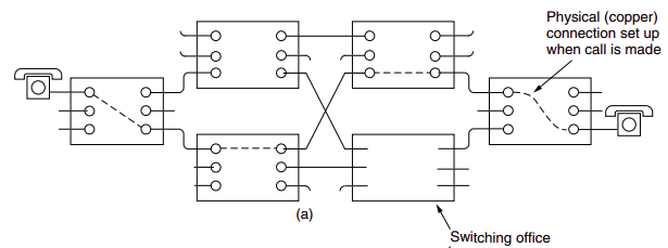
Packet switching

To send a message from a source end system to a destination end system, the source breaks long messages into smaller chunks of data known as packets. Between source and destination, each packet travels through communication links and packet switches (for which there are two predominant types, routers and link-layer switches). Packets are transmitted over each communication link at a rate equal to the full transmission rate of the link. So, if a source end system or a packet switch is sending a packet of L bits over a link with transmission rate R bits/sec, then the time to transmit the packet is L /R seconds.

Most packet switches use store-and-forward transmission at the inputs to the links. Store-and-forward transmission means that the packet switch must receive the entire packet before it can begin to transmit the first bit of the packet onto the outbound link.

A router will typically have many incident links, since its job is to switch an incoming packet onto an outgoing link; in this simple example, the router has the rather simple task of transferring a packet from one (input) link to the only other attached link.

A router will typically have many incident links, since its job is to switch an incoming packet onto an outgoing link; in this simple example, the router has the rather simple task of transferring a packet from one (input) link to the only other attached link.

In the Internet, every end system has an address called an IP address. When a source end system wants to send a packet to a destination end system, the source includes the destination’s IP address in the packet’s header. As with postal addresses, this address has a hierarchical structure. When a packet arrives at a router in the network, the router examines a portion of the packet’s destination address and forwards the packet to an adjacent router. More specifically, each router has a forwarding table that maps destination addresses (or portions of the destination addresses) to that router’s outbound links.

The Internet has a number of special routing protocols that are used to automatically set the forwarding tables.

A packet is treated independently of all others. Same destination packets may travel different paths to reach their destination. The switching mechanism an cause the datagrams to arrive at their destination out of order with different delay.

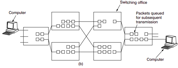
Circuit Switching

In circuit switched networks, the resources needed along a path (buffers, link transmission rate) to provide for communication between the end systems are reserved for the duration of the communication session between the end systems. In packet-swtiched networks, these resources are not reserved; a session’s messages uses the resources on demand, and as consequences, may have to wait for access to a communication link.

Traditional telephone networks are examples of circuit-switched network. Before the sender can send the information, the network must establish a connection between the sender and the receiver. When the network establishes the circuit, it also reserves a constant transmission rate in the network’s links (representing a fraction of each link’s transmission capacity) for the duration of the connection. In contrast, in packet-switched network, a packet is sent into the network without reserving any link resources whatsoever, if one of the links is congested because other packets need to be transmitted over the link at the same time, then the packet will have to wait in a buffer at the sending side of the transmision link and suffer a delay.

The proponents of packet switching have always argued that circuit switching is wasteful because the dedicated circuits are idle during silent periods; also that establishing end-to-end circuits and reserving end-to-end transmission capacity is complicated and requires complex signaling software to coordinate the operation of the switches along the end-to-end path. The critics of packet switching have often argued that packet switching is not suitable for real-time services because of its variables and unpredictable end-to-end delays, while proponents argue that it offers better sharing of transmission capacity than circuit switching and is more efficient, and less costly to implement.

Virtual-circuit networks

Cross between a circuit-switched and a data-gram network, Global address to create a virtual-circuit identifier with switch scope, Global addresses help switches make table entries for their connection, A packet arrives at a switch with a VCI and leaves with a different VCI. The setup request and the acknowledgement, Each switch that receives the setup request frame assigns the incoming port, chooses an available incoming VCI and the outgoing port, Does not yet know the outgoing VCI, which will be found during the acknowledgement step, Acknowledgement frame completes the entries in the switching tables, Established path is a virtual circuit, The switch looks in its table to find corresponding port and VCI. When it is found, the switch knows to change the VCI and send out accordingly -In the teardown phase, the source and destination inform the switches to delete the corresponding entry. A special frame called a teardown request sent by source. Destination responds with a teardown confirmation frame. All switches delete the corresponding entry from their tables

		>Efficiency:
			-In virtual-circuit switching, all packets belonging to the same source and destination travel the same path, but the packets may arrive at the destination with different delays if resource allocation is on demand
			-Source can check the availability of the resources, without actually reserving it
			-In a virtual-circuit network, there is a one-time delay for setup and a one-time delay for teardown. If resources are allocated during the setup phase, there is no wait time for individual packets
		
		>Example: Switching at the WAN is normally implemented by using virtual-circuit techniques. Probably LANs too.

INFORMATION THEORY:

>Entropy is a measure of quantified information in a random variable. It is a property of the probability distribution of a random variable, intuitively, the entropy Hx of a discrete random variable X is a measure of the amount of uncertainty associated with the value of X when only its distribution is known.
-It gives a limit on the rate at which data generated by independent samples with the given distribution can be compressed reliably

>Another useful concept is mutual information defined on two random variables, which describes the measure of information in common between those variables, which can be used to describe their correlation. The latter is a property of the joint distribution of two random variables, and is the maximum rate of reliable communication across a noisy channel in the limit of channel statistics that are determined by the joint distribution.

>Entropy of an information source:
	-Based on the probability mass function of each source symbol to be communicated, the Shannon entropy H, in units of bits (per symbol), is given by
			H = -S[pi lg(pi)]
		where, pi is the probability of occurence of the ith possible value of the source symbol. 
	-The choice of logarithmic base determines the unit of information entropy that is used. A common unit of information is the bit, based on the binary logarithm. 
	
>Entropy of a source that emits a sequence of N symbols that are independent and identically distributed is N.H bits (per message of N symbols). 
>Example: If one transmits 1000 bits (0s and 1s), and the value of each of these bits is known to the receiver (has a specific value with certainty) ahead of transmission, it is clear that no inforamtion is transmitted. If, however, each bit is independently equally likely to be 0 or 1, 1000 shannons of information (more often called bits) have been transmitted

>Between these two extremes, information can be quantified as follows.
		If X is the set of all messages {x1,..,xn} that X could be, and p(x) is the probability of some x in X, then the entropy, H, of X is defined as:
			H(X) = Expected value of [I(x)] = -S[p(x)log(p(x))]
		where, I(x) is the self-information, which is the entropy contribution of an individual message, and Ex is the expected value. 			
		
>A property of entropy is maximized when all the messages in the message space are equiprobable p(x) = 1/n; i.e., most unpredictable, in which H(x) = logn

>Self-information:
	-Quantity derived from the proability of a particular event occuring from a random variable. For an event x with probability P, the information content is defined as:
		I(x) = -lg[Pr(x)]
	-Meets the axioms:
		>An event with probability of 100% is perfectly unsurprising and yields no infomratin
		>The less probable an event is, the more surprising it is and the more information it yields.
		>If two independent events are measured separately, the total amount of information is the sum of the self-informations of the individual events.


>What to take away? 

Entropy:
	>uncertainty in information source
	(Higher the value, higher the spread of energy, higher the uncertainly in IS)

	>average number of bits required to represent the outcomes
	SUM over all i's [probability of ith * lg (1/probabitiy of ith)]
	
	Ex: the uniform distribution has the highest entropy in all the cases
	
Cross entropy:
	>
	
	>average number of bits required to represent outcomes from a information source when its mistaken	
	= SUM over all i's [ actual probability of ith * log (1/assumed probablity of ith)]
	
Hence, entropy provides measure for how information coming from a source can be compressed reliably without loss of information, so with this encoding we can certainly extract required information

CODING THEORY: >One of the most important and direct applications of information theory. Using a statistical description for data, information theory quantifies the number of bits needed to describe the data, which the information entropy of the source. Divided into: 1. Data compression (source coding) >Two formulations for the compression problem: -Lossless data compression: The data must be reconstructed exactly -Lossy data compression: Allocates bits needed to reconstruct the data, within a specified fidelity level measured by a distortion function

2. Error-correcting codes (channel coding)
	>While data compression removes as much redundancy as possible, an error-correcting code adds just the right kind of redundancy (i.e., error correction) needed to transmit the data efficiently and faithfully across a noisy channel.

SOURCE CODING: >A particular type of optimal prefix code that is commonly used for lossless data compression. When we encode data as binary patterns, we normally use a fixed number of bits for each symbol. To compress data, we can consider the frequency of symbols and the probability of their occurence in the message. Huffman coding assigns shorter codes to symbols that occur more frequently and longer codes to those that occur less frequently. >To use Huffman coding, we first need to create the Huffman tree. The Huffman tree is a tree in which the leaevs of the tree are the symbols. It is made so that the most frequent symbol is the closest to the root of the tree (with minimum number of notes to the root) and the least frequent symbol is farthest from the root. >Goto DSA

ERROR CORRECTION: >Any time data are transmitted from one node to the next, they can become corrupted in passage. Many factors can alter one or more bits of a message. Some applications require a mechanism for detecting and correcting errors >Central concept in detecting or correcting errors is redundancy. To be able to detect or correct errors, we need to send some extra bits with our data. These redundant bits are added by the sender and removed by the receiver. Their presence allows the receiver to detect or correct corrupted bits. >Redundancy is achieved through various coding schemes: block coding and convolution coding.

1. BLOCK CODING
	-We divide our message into blocks, each of k bits, called datawords. We add r redundant bits to each block to make the length n = k+r. The resulting n-bit blocks are called codewords.

	-Comment: k datawords, r redundancies, n codewords

	-With k bits, we can create a combination of 2^k datawords; with n bits, we can create a combination of 2^n codewords. Since n > k, the number of possible codewords is larger than the number of possible datawords. The block coding process is one-to-one; the same dataword is always encoded as the same codeword. This means that we have 2^n-2^k codewords that are not used
	-If the receiver receives an invalid codeword, this indicates that the data was corrupted during transmission

	ERROR DETECTION:
		>If the following two conditions are met, the receiver can detect a change in the original codeword
			-The receiver has (or can derive) a list of valid codewords.
			-The original codeword has changed to an invalid one
		> If the received codeword is the same as one of the valid codewords, the word is accepted; the corresponding dataword is extracted for use. If the received codeword is not valid, it is discarded. However, if the codeword is corrupted during transmission but the received word still matches a valid codeword, the error remains undetected.
		>An error-detecting code can detect only the types of errors for which it is designed; other types of errors may remain undetected
		>Rate of code is defined as ratio between its dataword length and codeword length.

	CODE METRICS:
		Hamming Distance:
		>The hamming distance d(x,y) between two words x and y (of the same size) is the number of differences between the corresponding bits.
		>Is the number of bits that are corrupted during transmission. If the HD between the sent and the received codeword is not zero, the codeword has been corrupted during transmission
			d(x,y) = no of 1's in [sent XOR received]

		>In a set of codewords, the minimum Hamming distance is the smallest Hamming distance between all possible pairs of (valid) codewords. If s errors occur during transmission, the Hamming distance between the sent codeword and received codword is s. 
		
		>If our system is to detect up to s errors, the minimum distance between the valid codes must be (s + 1), so that the received codeword does not match a valid codeword. Although a code with dmin = s + 1 may be able to detect more than s errors in some special cases, only s or fewer errors are guaranteed to be detected
		>k-error Detecting: a code C is said to be k error detecting if, and only if, the minimum Hamming distance between any two of its codewords is at least k+1
		>k-error Correction: a code C is said to be k error correcting if, and only if, the minimum Hamming distance between any two of its codewords is at least 2k+1

		>Properties:
			-Satisfies triangle inequality. Hamming distance between a and c is not larger than the sum of Hamming distance between a and b and between b and c. 

		Code rate:
		>The ratio between the number of informationa bits and the total number of bits (ie information plus redundancy bits) in a given communication package. 


	LINEAR BLOCK CODES:
		>Informally, a linear block code is a code in which exclusive OR (addition modulo-2) of two valid codwords creates another valid codword
		>Minimum Hamming distance is the number of 1s in the nonzero valid codeword with the smallest number of 1s.

		EX: PARITY-CHECK CODE: (FIGURE)
		>Intro: Most popular linear error-detecting code. In this code, a k-bit dataword is changed to an n-bit codeword where n = k+1. The extra bit, called the parity bit, is selected to make the total number of 1s in the codeword even. As the parity bit is inserted into the message, it is no longer special and becomes part of it.

		>Sender: The encoder uses a generator that takes a copy of 4-bit dataword and generates a parity bit r0. The dataword bits and the parity bit creates the 5-bit codeword. 
			r0 = a3+a2+a1+a0 (mod-2)

		>Receiver: The checker at the receiver does the same thing as the generator in the sender with one exception: The addition is done over all 5 bits. The result, which is called the syndrome, is just 1 bit. The syndrome is 0 when the number of 1s in the received codeword is even; otherwise, it is 1. 
			s0 = b3+b2+b1+b0+q0 (mod-2)

The syndrome is passed to the decision logic analyzer. If the syndrome is 0, there is no detectable error in the received codeword; the data portion of the received codeword is accepted as the dataword; if the syndrome is 1, the data portion of the received codeword is discarded.

		>Metrics: minimumHammingDistance = 2, codeRate = n/(n+1)


		EX: HAMMING CODE:
		>Intro: Key insight to implement parity bits for carefully selected subsets so by checking can pin down exact location of the error. Can correct any single-bit error, or detect all single-bit and two-bit errors. [More like pinning down the truth by asking yes/no questions]. Mathematically, Hamming codes are a class of binary linear code. For each interger r >= 2, there is a code-word with codeword (block) length n = 2^r-1 and dataword (message) length of k = 2^r-r-1. In coding theory, Hamming(7,4) is a linear error-correcting code that encodes four bits of data into seven bits by adding three parity bits.
		>Sender: Goal of sender in Hamming codes is to create a set of parity bits that overlap so that a single-bit error in a data bit or a prity bit can be detected and corrected. Which parity bits cover which transmitted bits in the encoded word and their location is given by mapping between each data and parity bit into its final bit position (1 through 7) as presented in a Venn diagram. (VENN DIAGRAM). As Hamming codes are linear codes, they can alternatively constructed using the Hamming matrices: 
			Generator(G) = [Ik | P]
				    1 0 0 0 1 0 1
				    0 1 0 0 1 1 1
				    0 0 1 0 1 1 0
				    0 0 0 1 0 1 1

		>Receiver: (even wala rule follow bhako bhaye do the XORing of all the position bits (harek bits ko position hunxa or 0 dinxa if there was no error) and you get your error location, watch 3b1b bro you need it) The receiver multiplies H and the received codeword to obtain the syndrome, which indicates whether an error has occured, and if so, for which codeword bit. If the syndrome is a null vector, the receiver can conclude that no error has occured. 
			Checker(H) = [P^T | In-k]
				    1 1 1 0 1 0 0
				    0 1 1 1 0 1 0
				    1 1 0 1 0 0 1
		Otherwise, we can write
			Received codeword = Actual codeword + error bit
		If we multiply this vector by H, Hr = H(x+ei) = Hei, which picks out the error column, so we know the place of error. 

		>Metrics: They achieve the highest possible rate for codes with their block length and minimum distance of three
				R = 1-r/(2^r-1)

		>Appilcations: Due to the limited redundancy that Hamming codes add to the data, they can only detect and correct errors when the error rate is low. This is the case in computer memory (usually RAM), where bit errors are extremely rare and Hamming codes are widely used. 

	CYCLIC CODES:
		>Intro: Special linear block codes with one extra property that if a codeword is cyclically shifted (rotated), the result is another codeword. A subset of cyclic codes called cyclic redundancy check (CRC) is used in networks such as LANs and WANs.  
		>Sender: In the encoder, the dataword has k bits (say 4); the codeword has n bits (say 7, commet: jati ni huna sakxa sayad yo ta but then divisor ko size paila choose garinxa jasle yeslai fix gardinxa). The size of the dataword is augmented by adding n-k (3 here) 0s to the right-hand side of the word. The n-bit result is fed into the generator which uses modulo-2 division with divisor of size n-k+1 (4 here), predefined and agreed upon. The quotient of the dvision is discarded; the remainder is appended to the dataword to create the codeword. 
		>Receiver: The decoder receives the codeword (possibly corrupted in transistion). A copy of all n bits is fed to the checker, which is a replica of generator. The remainder producced by the checker is a syndrome of n-k (3 here) bits, whcih is fed to the decision logic analyszer. If the syndrome bits are all 0s, the 4 left-most bits of the codeword are accepted as the dataword (interpreted as no error); otherwise, the 4 bits are discarded (error). For data word 1001 (9, bit-size 4) and divisor 1011 (11, bit-size 4). So the code word will be 7-bit in size. The remainder is 110 (6). Codeword is 1001110
		
		>POLYNOMIALS:
			-A pattern of 0s and 1s can be represented as a polynomial with coefficients of 0 and 1. The power of each term shows the position of the bit; the coefficient shows the value of the bit. Simplifies the codeword generation.
			-To find the augmented dataword, left-shift dataword by 3 bits (multiplying by x^3). Division is straight forward
			-Polynomial representation can easily simplify the operation of division in this case, because the two steps involving all-0's divisors are not needed here. In a polynomial representation, the divisor is normally referred to as the generator polynomial t(x)
			-Say: Dataword:d(x), Codword:c(x), Generator:g(x), Syndrome:s(x), Error:e(x)
			-If s(x) != 0, one or more bits is corrupted. Else, no bit is corrupted, or some bits are corrupted, but the decoder failed to detect them


			-Impose criteria that must be imposed on the generator, g(x) to detect the type of error we specially want to be detected. 
				Sent codeword = c(x)
				Received codeword = c(x)+e(x)
			-Receiver divides codeword by g(x) to get the syndrome:
				Syndrome = Remainder of e(x)/g(x)
			-Those errors that are divisible by g(x) are not caught

			1. Single-bit error [Euta matra error]
				-A single-bit error is e(x)=x^i, where i is the position of the bit. If a single-bit error is caught, then x^i is not divisible by g(x). 
				-If g(x) has at least two terms (which is normally the case) and coefficient of constant term is not zero (the rightmost bit is 1), then e(x) cannot be divided by g(x)
		
			2. Odd numbers of errors [Odd number ota error]
				-A generator that contains a factor of x+1 can detect all odd-numbered errors.
			
			3. Two isolated single-bit errors [Duita matra errors]
				-Error of this type as e(x) = x^j+x^i (j>i). Can write as x^i[x^(j-1)+1]. If g(x) can detect single-bit error and cannot divide x^t+1 (t between 0 and n-1), then all isolated double errors can be detected.

			4. Burst errors [More than duita]
				-A burst error is of form e(x) = x^j+...+x^i. Can factor out x^i as x^i[x^(j-i)+...+1]. If our generator can detect a single error, then it cannot divide x^i. Worry is about the generators that divide x^(j-1)+...+1. Say generator is x^r+...+1. Then the remainder of [x^(j-1)+...+1]/[x^r+...+1] must not be zero. 
				-If $j-r < r$, the remainder can never be zero. Letting j-i = L-1 where L is the length of the error. This means all burst errors with length smaller than or equal to the number of check bits (r+1) will be detected. (meaning that burst error of size less than degree of divisor polynomial are caught rey)
				-In some rare cases, if j-i = r, L = r+1, the syndrome is 0 and the error is undetected. The probability of undetected burst error of length r+1 is (1/2)^(r-1)
				-In some rare cases, if j-i > r, L > r+1, the syndrome is 0 and the error is undetected. The probability of undetecting such errors is (1/2)^r

			-Standard polynomials:
				CRC-3: x^3+x+1
				CRC-4: x^4+x+1
				CRC-5-USB: x^5+x^2+1
				CRC-5-ITU: x^5+x^4+x^2+1
					-(See if batches one bit errors, burst error of size less than 5 are caught while highers have some probabilities, give example of each)
			-Hardware:
				-Fixed hardwired divisor for cyclic if we know the divisor pattern. Registers to hold bits. 

2. CONVOLUTION CODES:
	>Background: A type of error-correcting code that generates parity symbols via sliding application of a boolean polynomial function to a data stream. The sliding application represents the convolution of the encoder over the data, which gives rise to the term convolutional coding. The sliding nature of the convolutional codes faciliates trellis decoding using a time-invariant trellis. The maximum likelihood soft decision decoding is one the major benefits of convolution codes. This is in contrast to classic block codes, which are represented by time-variant trellis and therefore are typically hard-decision decoded.

	>Intro: Convolution codes are often characterized by the base code rate and the depth (or memory) of the encoder [n,k,K]. The base code rate is typicaly given as k/n, where k is the raw input data rate and k is the data rate of output channel encoded stream. The memory is often called the constraint length K, (yo chai number of states sanga related hunxa) where the output is a function of the current input as well as the previous K-1 inputs. The code rate of a convolution code is commonly modified via symbol puncturing. For example, a convolutional code with a 'mother' code rate n/k=1/2 may be punctured to a higher rate of, for example, 7/8 simply by not transmitting a portion of code symbols.

	>Sender: To convolutionaly encode data, start with K or lg(number of states) memory registers, each holding one input bit. Unless specified, all memory registers start with a value of 0. The encoder has n (output rate, input rate is taken as 1) modulo-2 adders, and n generator polynomials- one for each adder. Using the generator polynomials and the existing values in the remaining registers, the encoder outputs n symbols. These symbols may be transmitted or punctured depending on the desired code rate. Now bit shift all register values to the right (m1 moves to m0, m0 moves to m−1) and wait for the next input bit. If there are no remaining input bits, the encoder continues shifting until all registers have returned to the zero state (flush bit termination).

	>Receiver: A convolution encoder is a finite state machine. An encoder with n binary cells will have 2^n states. An actual encdoed sequence can be represented as a path on the Trellis diagram (yo diagram chai kati ota bit check garni ho tesma depend garxa). The diagram gives us an idea about decoding: if a received sequence does not fit this graph then it was received with errrors and we must choose the nearest correct sequence. The real decoding algorithms expoit this idea. Several algorithms exist for decoding convolution codes. For relatively small values of k, the Viterbi algorithm is universaly used as it provides maximum likelihood performance and is highly parallelizable

Information System

6. Data rate limits:

   Data rate is how fast we can send data, in bits per second, over a channel. Depends on -The bandwidth available -The quality of the channel -The levels of signals we use (probably the modulation technique) Two theoretical formulas were developed to calculate the data rate.

   1. Shannon’s capacity: The channel capacity, meaning the theoretical tighest upper bound on the information rate of data that can be communicated at an arbitarliy low error rate using an average received power S through an analog communication channel of bandwidth B, subject to additive white Gaussian noise of power N: BitRate = B x log_2(1+S/N)

      Shows how to computer a channel capacity from a statistical description of a channel, and establishes that given a noisy channel with capacity C and information transmitted at a line rate R, then if -$R<C$, there exists a coding technique which allows the probability of error at the receiver to be made arbitrarily small -R > C, the probability of error at the receiver increases without bound as the rate is increased. So no useful information can be transmitted beyond the channel capacity

      NOTE: If there were such a thing as a noise-free analog channel, one could transmit unlimited amounts of error-free data over it per unit of time. The Nyquist formula tells how many signals levels are needed given we use PCM.

   2. Noiseless channel: Nyquist bit rate formula (supposedly) defines the theoretical maximum bit rate of implicity assumed noiseless channel BitRate = 2Bandwidthlog_2(L) According to the formula, given a specific bandwidth, we can have any bitrate we want by increasing the number of signal levels. Although the idea is theoretically correct, practically when we increase the number of signal levels, we impose a burden on the receiver. It does not (itself) say that if these bits would be received reliably at the receiver in the presence of noise of channel distortion

Multiplexing

BANDWIDTH UTILLIZATION:

>Multiplexing is the set of techniques that allow the simultaneous transmission of multiple signals across a single data link. We can accomodate the traffic increase by continuing to add individual links each time a new channel is needed; or we can install higher-bandwidth links and use each to carry multiple signals
>In a multiplexed system, n lines share the bandwidth of one link. The lines on the left direct their transmission stream to a multiplexer, which combines them into a single stream (many-to-one). At the receiving end, that stream is fed into a demultiplexer, which separates the stream back into its componen transmission (one-to-many) and directs them to their corresponding lines. 
>Link refers to the physical path. Channel refers to the portion of a link that carries a transsmission between a given pair of lines.
>There are three basic multiplexing techniques:

1. Frequency-Division Multiplexing: (Horiziontal striips)
	(for air and other analog lines so uses any-analog modulation) Frequency-division multiplexing (FDM) 		
	>An analog technique that can be applied when the bandwidth of a link (in hertz) is greater than the combined bandwidths of the signals to be transmitted.
	>An analog multiplexing technique; however, this does not mean that FDM cannot be used to combine sources sending digital signals
		-Signals generated by each sending device modulate different carrier frequencies
		-These modulated signals are then combined into a single composite signal that can be transported by the link that has enough bandwidth to accommodate it

		-At the receiving end, series of bandpass filters to decompose the multiplxed into its constitutent component signals
		-Then individual signals are passed to a demodulator that separates them from their carrier and pass to ouptut lines
		-Channels can be separated by strips of unused bandwidth—guard bands—to prevent signals from overlapping


2. Wavelength-division multiplexing:
	>Designed to use the high data rate capability of fiber-optic cable The optical fiber data rate is higher than data rate of metallic transmission calbe, but using a fiber cable for single line wastes the available bandwidth.
	>Conceptually same as FDM except that the multiplexing and demultiplexing involve optical signals transmitted through fiber-optic channels. The idea is the same: We are combining different signals of different frequencies. The difference is that the frequencies are very high.
	>Although WDM technology is very complex, the basic idea is very simple. We want to combine multiple light sources into one single light at the multiplexer and do the reverse at the demultiplexer. The combining and splitting of light sources are easily handled by a prism as the prism bends a beam of light based on the angle of incidence and the frequency.
	
3. Time-dviision multiplexing: (Vertical strips)
	>A digital process that allows several connections to share the high bandwidth of a link. Instead of sharing a portion of the bandwidth as in FDM, time is shared.
	>Digital data from different sources are combined into one timeshared link. This does not mean that the sources cannot produce analog dadta; analog data can be sampled, changed to digital data, and then multiplexed by using TDM.
	
	SYNCHRONOUS: 
		>Each input connection has an allotment in the output even if is not sending data. The data flow of each input connection is divided into units, where each input occupies one input slot. A unit can be 1 bit, one character, or one block of data. Each input uint becomes one output unit and occupies one output time slot. However, the duration of an output time slot is n times shorter that the duration of an input time slot. If an input time slot is Ts, the output time slot is T/n s, where n is the number of connections. In other words, a unit in the output connection has a shorter duration; it travels faster.
	>In synchronous, a round of data from each unit conenction is collected in a frame. If we have n conenctions a frame is divided into n time slots so data rate of the output link must be n times the data rate of a connection to guarantee the flow of data.
	>Interleaving: TDM visualized as two oppositely rotating switches at same speed. On the multiplexing side, as the switch opens in front of a connection, that connection has the opportunity to send a unit onto the path. This prcess is interleaving. On demultiplexing side, as the switch opens the front of a conention has the opportuunity to receive a unit from the path
	>Emtpy slots: If a source does not have data to send, the correpsonding slot in the output frame is empty; 
	>Data Rate disparity: How to handle a disparity in the input data rates. Assumption was that the data rates of all input lines were the same. Three strategies: multilevel multiplexing, multiple-slot allocation, and pulse stuffing
	

	STATISTICAL:  
		>In statistical time-division multiplexing, slots are dynamically allocated to improve bandwidth efficiency. The multiplexer checks each input line in roundrobin fashion; it allocates a slot for an input line if the line has data to send; otherwise, it skips the line and checks the next line. In output slot in synchronous TDM is totally occupied by data; in statistical TDM, a slot needs to carry data as well as the address of the destination.

4. CDMA:
	>Some textbooks consider CDMA as a fourth multiplexing category, we discuss CDMA as an access metho		

Comment: Multiplexing was to combine signals to form a larger bandwidth, now we just increase bandwidth like an idiot?

HANNELIZATION: [High on the OSI] A multiple-access method in which the available bandwidth of a link is shared in time, frequency, or through code, among different stations

CDMA differs from FDMA in that only one channel occupies the entire bandwidth of the link. It differs from TDMA in that all stations can send data simultaneously; there is not timesharing
 
>Idea: 
	-Same room, different language
	-For four stations d1, d2, d3, d4 (usually power of 2) connected to same channel. The data from station 1 are d1, from station 2 are d2, and so on. The code assigned to the first station is c1, to the second c2, and so on.
	-Assume that the assigned codes have two properties:
			>If we multiply each code by another, we get 0
			>If we multiply each code by itself, we get 4 (the number of stations)

	-Each station is assigned a code, which is a orthogoal sequence of numbers called chips
		>Each sequence is made of N elements, where N is the number of stations				>If we multiply a sequence by a number, every element in the sequence is mulitiplied by that element
		>If we multiply two equal sequences, element by element, and add the results, we get N, where N is the number of elements in each seqeunce. Called inner product
		>If we multiply two diferent sequences, element by element, and add the results, we get 0. This is called inner product of two different sequences.	
		>Adding two seqeunces means adding the corresponding elements. The result is another sequence
	-To generate chip sequences, we use a Walsh table (or a matrix). If we know the table for N sequences W(N), we can create the table for 2N sequences, W(2N). Can be calcualted recursively as:
		W(1) = [+1], W(2N) = [W(N) W(N) ]
				      [W(N) W(N)']

>Data transfer
	-Station 1 mulitplies its data by its code to get d1.c1. Station 2 multiplies it data by its code to get d2.c2, and so on. 
	-The data that go on the channel are the sum of all the terms.
	-Any station that wants to receive data from one of the other three multiplies the data on the channel by the code of the sender
	-If stations 1 and 2 are talking to each other. Station 2 wants to hear what station 1 is saying. It mutiplies the data on the channel by c1, the code of station 1. Because c1.c1 is 4, but c2.c1, c3.c1, c4.c1 are all 0s, station 2 divides the result by 4 to get the data from station 1. 
 	-If a stations needs to send a 0 bit, it encodes it as -1; and if it needs to send a 1 bit, it encodes it as +1. When a station is idle, it sends no signal, which is interpreted as a 0	
	-Stations 1 and 2 are sending a 0 bit and channel 4 is sending a 1 bit. Station 3 is silent. 
 	-Each station multiplies the corresponding number by its chip, whcih is unique for each station.
		-d1.c1 = -1*[1  1  1  1]
		-d2.c2 = -1*[1 -1  1 -1]
		-d3.c3 = +0*[1  1 -1 -1]
		-d4.c4 = +1*[1 -1 -1  1]

SPREADING:

	>Is an extension to multiplexing that combines signals from diferent sources to fit into a larger bandwidth, but with aim to avoid interference and interception.
	>Used in wireless applications with security concerns that outweight bandwidth efficiency. In wireless, all stations use air (or a vacuum) as the medium for communication. Stations must be able to share this medium without interception by an eavesdropper and without being subject to jamming from a malicious intruder. 
	>Achieves its goals through two principles:
		-Bandwidth allocated to each station needs to be, by far, larger than what is needed. This allows redundancy
		-The expanding of the original bandwidth B to the bandwidth Bss must be done by a process that is independent of the original signal. In other words, the spreading process occurs after the signal is created by the source. 
	
>Two techniuqes:

1. FHSS:
	>Uses M different carrier frequencies that are modulated by the source signal. At one moment, the signal modulates one carrier frequency; at next; modulates another carrier frequency. Althrough done using one carrier at a time, M frequencies are used in the long run. The bandwidth occupied by a source after spreading is BFHSS >> B
	>A pseudorandom noise injects a k-bit pattern for every hopping period Th. (Pseudorandom means that the pattern is repeated after the hopping period) The frequency table uses the pattern to find the fequency to used for this hopping period and passes it to the frequency synthesizer. 
	>The frequency table uses the pattern to find the freq to be used for this hopping period and passes it to synthesizer. The frequency synthesizer creates a carrier signal of that frequency and source signal modulates the carrier signal.
	>Suppose we have decided to have eight hopping frequencies. The pseudorandom code generator will create eight different 3-bit patterns. These are mapped to eight different frequencies in the frequency table. 

	>ADVANTAGES:
		-Now if hopping period is short, an intruder tries to intercept the transmitted singal, they can only access a small piece of data because she does not know the spreading sequence to quickly adapt herself to the next hop.
		-Antijamming mechanism as a malicious sender may be able to send noise to jam the singal for one hopping period (randomly)
		-Prevents electromagnetic interference preserving signal integrity

	>BANDWIDTH SHARING:
		-If the number of hopping frequencies is M, we can multiplex M channels into one by using the same Bss bandwidth. This is because a station uses just one frequency in each hopping period; M-1 other frequencies can be used by M-1 other stations.  In other words, M different stations can use the same Bss if an appropriate modulation technique such as multiple FSK is used. FHSS is similar to FDM. 
	
2. DSSS: (To include or not)
	>Expands the bandwidth of the original signal, whereby we replace each data bit with n bits using a spreading code. In other words, each bit is assigned a code of n bits, called chips, where the chip rate is n times that of the data bit. 
	>Used in wireless LAN, the famous Barker sequence, where n is 11: 10110111000. This means that the required bandwidth for the spread signal is 11 times larger than the bandwidth of the original signal.
	>The data is bit-wise XORed with the Barker sequence 
	
	>BANDWIDTH SHARING:
		-If we use a spreading code that spreads signals (from different stations) that cannot be combined and separated, we cannot share a bandwidth. However, if we use a special type of sequence code that allows the comibing and separating of spread signals, we can share the bandwidth

Error-detection and correction techniques

-(transport le ni garthyo haina ra?)
-At the sending side, data, D, to be protected against but errors is augmenetd with error-detection and -correction bits (EDC), includes not only network layer datagram but also link-level addressing ifnroation, sequence numbers, and other fields in the frame header
-Both D and EDC are sent to the receiving node in a link-level frame, D' and EDC' is received which may differ from originals
-Go into three common ones:

1. Parity checks (basics)
	-Suppose that the information to be sent, D has d bits, the sender simply includes one additional bit and chooses its value such that the total number of 1s in the d+1 bits (the original inofmriaotn plus a partiy bit) is even
	-If the probabliity of bit errors is small and errors can be assumed to occur independently from one bit to the next, the probabliilty of multiple bit errosr in a packet would be extremely small
	-Measurements have shown that, rather than occuring independently, errors are often clustered together in bursts, under which if partity is used undetected errors go upto 50%

2. Checksumming methods (at tranports layer)
	-Require relatively little packet overhead, checksums in TCP and UDP use only 16 bits, however provide relativley weak protection against errors as compared with cyclic redundancy check
	-A 16 bit sum of words checksum will detect all single bit errors and all error bursts of length 16 bits or fewer
	-Why checksum at transport and CRC at hardware? recall that transport layer is implemented in software, important to have a simple and fast error-detection schehe such as checksumming
	-While at link layer is dedicated hardware in adapters, which can rapidly perofrm more complex CRC operations
	
	
3. CRC (at link)
	-read theory later

Bandwidth

The term bandwidth refers to the channel capacity of a logical or physical communication path in a digital communication system.

The maximum rate that can be sustained on a link is limited by the Shannon channel capacity for these communication systems which is dependent on the bandwidth in hertz and the noise on the channel.

Latency

As a packet travels from one node (host or router) to the subsequent node (host or router) along this path, the packet suffers from several types of delays at each node along the path.

The most important of these delays are the nodal processing delay, queuing delay, transmission delay, and propagation delay; together, these delays accumulate to give a total nodal delay.

When the packet arrives at a router from the upstream node, it examines the packet’s header to determine the appropriate outbound link for the packet and then directs the packet to this link.

1. Processing: The time required to examine the packet’s header and determine where to direct the packet is part of the processing delay. The processing delay can also include other factors, such as the time needed to check for bit-level errors in the packet that occurred in transmitting the packet’s bits from the upstream node.

2. Queuing: At the queue, the packet experiences a queuing delay as it waits to be transmitted onto the link. The length of the queuing delay of a specific packet will depend on the number of earlier-arriving packets that are queued and waiting for transmission onto the link. If the queue is empty and no other packet is currently being transmitted, then our packet’s queuing delay will be zero. On the other hand, if the traffic is heavy and many other packets are also waiting to be transmitted, the queuing delay will be long.

3. Transmission: Denote the length of the packet by $L$ bits, and denote the transmission rate of the link from by $R$ bits/sec. For example, for a $10$ Mbps Ethernet link, the rate is for a $100$ Mbps Ethernet link, the rate is $R=100$Mbps. The transmission delay is $L/R$. This is the amount of time required to push (that is, transmit) all of the packet’s bits into the link. Transmission delays are typically on the order of microseconds to milliseconds in practice.

4. Propagation: Once a bit is pushed into the link, its needs to propagate to the other node. Time to propagate from the beginning of the link to it’s end is called the propagation delay. The propagation speed depends on the physical medium of the link and is, or little less than, the speed of light.

Packet Loss

The most complicated component of nodal delay is the queuing delay. Let $a$ denote the average rate at which packets arrive at the queue (a is in units of packets/sec). Recall that R is the transmission rate; that is, it is the rate (in bits/sec) at which bits are pushed out of the queue. Also suppose, for simplicity, that all packets consist of L bits. Assume that the queue is very big, so that it can hold essentially an infinite number of bits. The ratio La/R, called the traffic intensity, often plays an important role in estimating the extent of the queuing delay. If La/R > 1, then the average rate at which bits arrive at the queue exceeds the rate at which the bits can be transmitted from the queue. In this unfortunate situation, the queue will tend to increase without bound and the queuing delay will approach infinity! Therefore, one of the golden rules in traffic engineering is: Design your system so that the traffic intensity is no greater than 1.

In particular, if the traffic intensity is close to zero, then packet arrivals are few and far between and it is unlikely that an arriving packet will find another packet in the queue. Hence, the average queuing delay will be close to zero. On the other hand, when the traffic intensity is close to 1, there will be intervals of time when the arrival rate exceeds the transmission capacity (due to variations in packet arrival rate), and a queue will form during these periods of time; when the arrival rate is less than the transmission capacity, the length of the queue will shrink.

In reality a queue preceding a link has finite capacity, although the queuing capacity greatly depends on the router design and cost. Because the queue capacity is finite, packet delays do not really approach infinity as the traffic intensity approaches 1. Instead, a packet can arrive to find a full queue. With no place to store such a packet, a router will drop that packet; that is, the packet will be lost.

Throughput

In addition to delay and packet loss, another critical performance measure in computer networks is end-to-end throughput. To define throughput, consider transferring a large file from Host A to Host B across a computer network. This transfer might be, for example, a large video clip from one peer to another in a P2P file sharing system. The instantaneous throughput at any instant of time is the rate (in bits/sec) at which Host B is receiving the file. If the file consists of F bits and the transfer takes T seconds for Host B to receive all F bits, then the average throughput of the file transfer is F/T bits/sec.

For some applications, such as Internet telephony, it is desirable to have a low delay and an instantaneous throughput consistently above some threshold (for example, over 24 kbps for some Internet telephony applications and over 256 kbps for some real-time video applications).

For other applications, including those involving file transfers, delay is not critical, but it is desirable to have the highest possible throughput.

Bandwidth-delay product

Number of bits that can fill the link.

Jitter

When different packets encounter different delays.