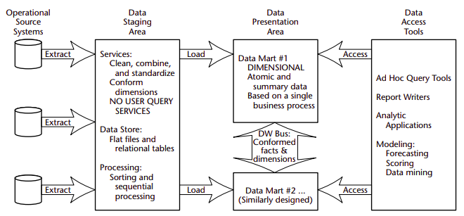
Operational source systems:
These are the operational systems of record that capture the transactions of the business. The source systems should be thought of as outside the data warehouse because presumably we have little to no control over the content and format of the data in these operational legacy systems. Queries against source systems are narrow, one-record-at-a-time queries that are part of the normal transaction flow and severely restricted in their demands on the operational system. The source systems maintain little historical data, and if you have a good data warehouse, the source systems can be relieved of much of the responsibility for representing the past.
Data staging area:
The data staging area of the data warehouse is both a storage area and a set of processes commonly referred to as extract-transformation-load (ETL). The data staging area is everything between the operational source systems and the data presentation area. It is somewhat analogous to the kitchen of a restaurant, where raw food products are transformed into a fine meal. In the data warehouse, raw operational data is transformed into a warehouse deliverable fit for user query and consumption.
Extraction is the first step in the process of getting data into the warehouse environment. Extracting means reading and understanding the source data and copying the data needed for the data warehouse into the staging area for further manipulation. Once the data is extracted to the staging area, there are numerous potential transformations, such as cleansing the data (correcting misspellings, resolving domain conflicts, dealing with missing elements, or parsing into standard formats), combining data from multiple sources, deduplicating data, and assigning warehouse keys. These transformations are all precursors to loading the data into the data warehouse presentation area.
Unfortunately, there is still considerable industry consternation about whether the data that supports or results from this process should be instantiated in physical normalized structures prior to loading into the presentation area for querying and reporting. These normalized structures sometimes are referred to in the industry as the enterprise data warehouse.
The data staging area is dominated by the simple activities of sorting and sequential processing. In many cases, the data staging area is not based on relational technology but instead may consist of a system of flat files. After you validate your data for conformance with the defined one-to-one and many-to-one business rules, it may be pointless to take the final step of building a fullblown third-normal-form physical database.
Data presentation:
The data presentation area is where data is organized, stored, and made available for direct querying by users, report writers, and other analytical applications. We typically refer to the presentation area as a series of integrated data marts. A data mart is a wedge of the overall presentation area pie. In its most simplistic form, a data mart presents the data from a single business process.
First of all, we insist that the data be presented, stored, and accessed in dimensional schemas. Our second stake in the ground about presentation area data marts is that they must contain detailed, atomic data. Atomic data is required to withstand assaults from unpredictable ad hoc user queries.
If the presentation area is based on a relational database, then these dimensionally modeled tables are referred to as star schemas. If the presentation area is based on multidimensional database or online analytic processing (OLAP) technology, then the data is stored in cubes. Contrary to the original religion of the data warehouse, modern data marts may well be updated, sometimes frequently. Incorrect data obviously should be corrected.
Data access tools:
The final major component of the data warehouse environment is the data access tool(s). We use the term tool loosely to refer to the variety of capabilities that can be provided to business users to leverage the presentation area for analytic decision making. By definition, all data access tools query the data in the data warehouse’s presentation area. A data access tool can be as simple as an ad hoc query tool or as complex as a sophisticated data mining or modeling application. Ad hoc query tools, as powerful as they are, can be understood and used effectively only by a small percentage of the potential data warehouse business user population.
Vocabulary
Fact Table:
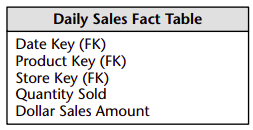
A fact table is the primary table in a dimensional model where the numerical performance measurements of the business are stored. We strive to store the measurement data resulting from a business process in a single data mart. We use the term fact to represent a business measure. We can imagine standing in the marketplace watching products being sold and writing down the quantity sold and dollar sales amount each day for each product in each store. A measurement is taken at the intersection of all the dimensions (day, product, and store). This list of dimensions defines the grain of the fact table and tells us what the scope of the measurement is.
A row in a fact table corresponds to a measurement. A measurement is a row in a fact table. All the measurements in a fact table must be at the same grain.
The most useful facts are numeric and additive, such as dollar sales amount.
It is very important that we do not try to fill the fact table with zeros representing nothing happening because these zeros would overwhelm most of our fact tables. By only including true activity, fact tables tend to be quite sparse.
We often describe facts as continuously valued mainly as a guide for the designer to help sort out what is a fact versus a dimension attribute. It is theoretically possible for a measured fact to be textual; however, the condition arises rarely. In most cases, a textual measurement is a description of something and is drawn from a discrete list of values.
All fact table grains fall into one of three categories:
- transaction,
- periodic snapshot,
- accumulating snapshot.
The fact table itself generally has its own primary key made up of a subset of the foreign keys. This key is often called a composite or concatenated key. Every fact table in a dimensional model has a composite key, and conversely, every table that has a composite key is a fact table. Another way to say this is that in a dimensional model, every table that expresses a many-to-many relationship must be a fact table. All other tables are dimension tables.
Fact tables express the many-to-many relationships between dimensions in dimensional models.
Dimension Tables:
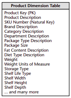
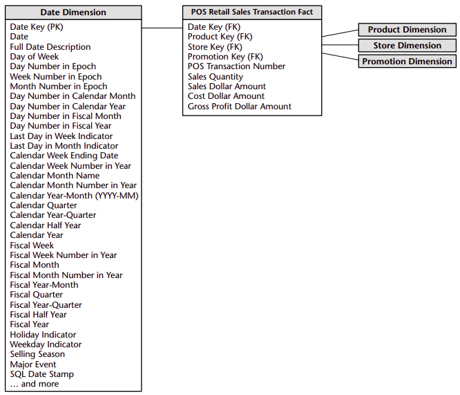
Dimension tables are integral companions to a fact table. The dimension tables contain the textual descriptors of the business. Dimension tables are integral companions to a fact table. The dimension tables contain the textual descriptors of the business. We strive to include as many meaningful textlike descriptions as possible. It is not uncommon for a dimension table to have 50 to 100 attributes. Dimension tables tend to be relatively shallow in terms of the number of rows (often far fewer than 1 million rows) but are wide with many large columns. Each dimension is defined by its single primary key, designated by the PK notation in our example which serves as the basis for referential integrity with any given fact table to which it is joined.
Dimension attributes serve as the primary source of query constraints, groupings, and report labels. In a query or report request, attribute are identified as the by words. For example, when a user states that he or she wants to see dollar sales by week by brand, week and brand must be available as dimension attributes.
Dimension table attributes play a vital role in the data warehouse. Since they are the source of virtually all interesting constraints and report labels, they are key to making the data warehouse usable and understandable. In many ways, the data warehouse is only as good as the dimension attributes. The power of the data warehouse is directly proportional to the quality and depth of the dimension attributes. The more time spent providing attributes with verbose business terminology, the better the data warehouse is. The more time spent populating the values in an attribute column, the better the data warehouse is. The more time spent ensuring the quality of the values in an attribute column, the better the data warehouse is.
Dimension tables are the entry points into the fact table. Robust dimension attributes deliver robust analytic slicing and dicing capabilities. The dimensions implement the user interface to the data warehouse.
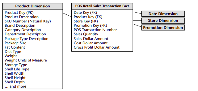
The best attributes are textual and discrete. Attributes should consist of real words rather than cryptic abbreviations. Typical attributes for a product dimension would include a short description (10 to 15 characters), a long description (30 to 50 characters), a brand name, a category name, packaging type, size, and numerous other product characteristics. Although the size is probably numeric, it is still a dimension attribute because it behaves more like a textual description than like a numeric measurement. Size is a discrete and constant descriptor of a specific product.
Sometimes when we are designing a database it is unclear whether a numeric data field extracted from a production data source is a fact or dimension attribute. We often can make the decision by asking whether the field is a measurement that takes on lots of values and participates in calculations (making it a fact) or is a discretely valued description that is more or less constant and participates in constraints (making it a dimensional attribute). For example, the standard cost for a product seems like a constant attribute of the product but may be changed so often that eventually we decide that it is more like a measured fact. Occasionally, we can’t be certain of the classification. In such cases, it may be possible to model the data field either way, as a matter of designer’s prerogative.
(like service ko cost fixed hunxa ki change hunxa brother?)
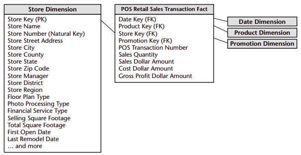
We strive to minimize the use of codes in our dimension tables by replacing them with more verbose textual attributes. We understand that you may have already trained the users to make sense of operational codes, but going forward, we’d like to minimize their reliance on miniature notes attached to their computer monitor for code translations. We want to have standard decodes for the operational codes available as dimension attributes so that the labeling on data warehouse queries and reports is consistent. We don’t want to encourage decodes buried in our reporting applications, where inconsistency is inevitable. Sometimes operational codes or identifiers have legitimate business significance to users or are required to communicate back to the operational world. In these cases, the codes should appear as explicit dimension attributes, in addition to the corresponding user-friendly textual descriptors. We have identified operational, natural keys in the dimension figures.
Operational codes often have intelligence embedded in them. For example, the first two digits may identify the line of business, whereas the next two digits may identify the global region. Rather than forcing users to interrogate or filter on the operational code, we pull out the embedded meanings and present them to users as separate dimension attributes that can be filtered, grouped, or reported on easily.
Dimension tables often represent hierarchical relationships in the business. In our sample product dimension table, products roll up into brands and then into categories. For each row in the product dimension, we store the brand and category description associated with each product. We realize that the hierarchical descriptive information is stored redundantly, but we do so in the spirit of ease of use and query performance. We resist our natural urge to store only the brand code in the product dimension and create a separate brand lookup table. This would be called a snowflake. Dimension tables typically are highly denormalized. They are usually quite small (less than 10 percent of the total data storage requirements). Since dimension tables typically are geometrically smaller than fact tables, improving storage efficiency by normalizing or snowflaking has virtually no impact on the overall database size. We almost always trade off dimension table space for simplicity and accessibility.
Bringing together facts and dimensions:
Now that we understand fact and dimension tables, let’s bring the two building blocks together in a dimensional model. The fact table consisting of numeric measurements is joined to a set of dimension tables filled with descriptive attributes. This characteristic starlike structure is often called a star join schema.
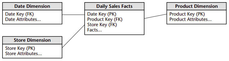
The first thing we notice about the resulting dimensional schema is its simplicity and symmetry. Obviously, business users benefit from the simplicity because the data is easier to understand and navigate.
The simplicity of a dimensional model also has performance benefits. Database optimizers will process these simple schemas more efficiently with fewer joins. A database engine can make very strong assumptions about first constraining the heavily indexed dimension tables, and then attacking the fact table all at once with the Cartesian product of the dimension table keys satisfying the user’s constraints. Amazingly, using this approach it is possible to evaluate arbitrary n-way joins to a fact table in a single pass through the fact table’s index.
Finally, dimensional models are gracefully extensible to accommodate change. The predictable framework of a dimensional model withstands unexpected changes in user behavior. Every dimension is equivalent; all dimensions are symmetrically equal entry points into the fact table. The logical model has no built-in bias regarding expected query patterns. There are no preferences for the business questions we’ll ask this month versus the questions we’ll ask next month. We certainly don’t want to adjust our schemas if business users come up with new ways to analyze the business.
We will see repeatedly in this book that the most granular or atomic data has the most dimensionality. Atomic data that has not been aggregated is the most expressive data; this atomic data should be the foundation for every fact table design in order to withstand business users’ ad hoc attacks where they pose unexpected queries. With dimensional models, we can add completely new dimensions to the schema as long as a single value of that dimension is defined for each existing fact row.
Likewise, we can add new, unanticipated facts to the fact table, assuming that the level of detail is consistent with the existing fact table. We can supplement preexisting dimension tables with new, unanticipated attributes. We also can break existing dimension rows down to a lower level of granularity from a certain point in time forward. In each case, existing tables can be changed in place either simply by adding new data rows in the table or by executing an SQL ALTER TABLE command. Data would not have to be reloaded. All existing data access applications continue to run without yielding different results.
Another way to think about the complementary nature of fact and dimension tables is to see them translated into a report. The dimension attributes supply the report labeling, whereas the fact tables supply the report’s numeric values.
Finally, as we’ve already stressed, we insist that the data in the presentation area be dimensionally structured. However, there is a natural relationship between dimensional and normalized models. The key to understanding the relationship is that a single normalized ER diagram often breaks down into multiple dimensional schemas. A large normalized model for an organization may have sales calls, orders, shipment invoices, customer payments, and product returns all on the same diagram. In a way, the normalized ER diagram does itself a disservice by representing, on a single drawing, multiple business processes that never coexist in a single data set at a single point in time. No wonder the normalized model seems complex.
If you already have an existing normalized ER diagram, the first step in converting it into a set of dimensional models is to separate the ER diagram into its discrete business processes and then model each one separately. The second step is to select those many-to-many relationships in the ER diagrams that contain numeric and additive nonkey facts and designate them as fact tables. The final step is to denormalize all the remaining tables into flat tables with singlepart keys that join directly to the fact tables. These tables become the dimension tables.
(some pitfalls, myths and all that good shift)
Four step dimensional design process:
-
Select the business process to model. A process is a natural business activity performed in your organization that typically is supported by a source data-collection system. Listening to your users is the most efficient means for selecting the business process. The performance measurements that they clamor to analyze in the data warehouse result from business measurement processes. Example business processes include raw materials purchasing, orders, shipments, invoicing, inventory, and general ledger. It is important to remember that we’re not referring to an organizational business department or function when we talk about business processes. For example, we’d build a single dimensional model to handle orders data rather than building separate models for the sales and marketing departments, which both want to access orders data. By focusing on business processes, rather than on business departments, we can deliver consistent information more economically throughout the organization. If we establish departmentally bound dimensional models, we’ll inevitably duplicate data with different labels and terminology. Multiple data flows into separate dimensional models will make us vulnerable to data inconsistencies. The best way to ensure consistency is to publish the data once. A single publishing run also reduces the extract-transformation-load (ETL) development effort, as well as the ongoing data management and disk storage burden.
-
Declare the grain of the business process. Declaring the grain means specifying exactly what an individual fact table row represents. The grain conveys the level of detail associated with the fact table measurements. It provides the answer to the question, “How do you describe a single row in the fact table?” Example grain declarations include:
- An individual line item on the customer’s retail sales ticket as measured by a scanner device
- A line item on a bill received from a doctor
- An individual boarding pass to get on a flight
- A daily snapshot of the inventory levels for each product in a warehouse
- A monthly snapshot for each bank account Data warehouse teams often try to bypass this seemingly unnecessary step of the process. Please dont! It is extremely important that everyone on the design tea is in agreement regarding the fact table granularity. It is virtually impossible to reach closure in step 3 without declaring the grain. We also should warn you that an inappropriate grain declaration will haunt a data warehouse implementation. Declaring the grain is a critical step that can’t be taken lightly
-
Choose the dimensions that apply to each fact table row. Dimensions fall out of the question, “How do businesspeople describe the data that results from the business process?” We want to decorate our fact tables with a robust set of dimensions representing all possible descriptions that take on single values in the context of each measurement. If we are clear about the grain, then the dimensions typically can be identified quite easily. With the choice of each dimension, we will list all the discrete, textlike attributes that will flesh out each dimension table. Examples of common dimensions include date, product, customer, transaction type, and status.
-
Identify the numeric facts that will populate each fact table row. Facts are determined by answering the question, “What are we measuring?” Business users are keenly interested in analyzing these business process performance measures. All candidate facts in a design must be true to the grain defined in step 2. Facts that clearly belong to a different grain must be in a separate fact table. Typical facts are numeric additive figures such as quantity ordered or dollar cost amount.
Retail sales
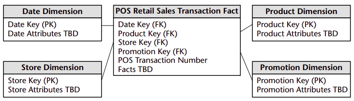
The first step in the design is to decide what business process(es) to model by combining an understanding of the business requirements with an understanding of the available data. The management wants to better understand customer purchases as captured by the POS system. Thus the business process we’re going to model is POS retail sales. The most granular data is an individual line item on a POS transaction. Once the grain of the fact table has been chosen, the date, product, and store dimensions fall out immediately. Of course, you can always declare higher-level grains for a business process that represent an aggregation of the most atomic data. However, as soon as we select a higher-level grain, we’re limiting ourselves to fewer and/or potentially less detailed dimensions.
The facts collected by the POS system include the sales quantity (e.g., the number of cans of chicken noodle soup), per unit sales price, and the sales dollar amount. The sales dollar amount equals the sales quantity multiplied by the unit price. Three of the facts, sales quantity, sales dollar amount, and cost dollar amount, are beautifully additive across all the dimensions. We can compute the gross profit by subtracting the cost dollar amount from the sales dollar amount, or revenue. Although computed, this gross profit is also perfectly additive across all the dimensions—we can calculate the gross profit of any combination of products sold in any set of stores on any set of days.
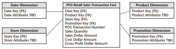
Percentages and ratios, such as gross margin, are nonadditive. The numerator and denominator should be stored in the fact table. The ratio can be calculated in a data access tool for any slice of the fact table by remembering to calculate the ratio of the sums, not the sum of the ratios. Unit price is also a nonadditive fact. Attempting to sum up unit price across any of the dimensions results in a meaningless, nonsensical number.
Although the POS transaction number looks like a dimension key in the fact table, we have stripped off all the descriptive items that might otherwise fall in a POS transaction dimension. Since the resulting dimension is empty, we refer to the POS transaction number as a degenerate dimension. Degenerate dimensions are very common when the grain of a fact table represents a single transaction or transaction line item because the degenerate dimension represents the unique identifier of the parent. Order numbers, invoice numbers, and bill-of-lading numbers almost always appear as degenerate dimensions in a dimensional model.
Dimensions:
The promotion dimension is potentially the most interesting dimension in our schema. The promotion dimension describes the promotion conditions under which a product was sold. Promotion conditions include temporary price reductions, end-aisle displays, newspaper ads, and coupons. This dimension is often called a causal dimension (as opposed to a casual dimension) because it describes factors thought to cause a change in product sales. Whether the products under promotion experienced a gain in sales during the promotional period. This is called the lift. The causal conditions potentially affecting a sale are not necessarily tracked directly by the POS system. The transaction system keeps track of price reductions and markdowns. The presence of coupons also typically is captured with the transaction because the customer either presents coupons at the time of sale or does not. Ads and in-store display conditions may need to be linked from other sources.
The various possible causal conditions are highly correlated. A temporary price reduction usually is associated with an ad and perhaps an end-aisle display. Coupons often are associated with ads. For this reason, it makes sense to create one row in the promotion dimension for each combination of promotion conditions that occurs. Over the course of a year, there may be 1,000 ads, 5,000 temporary price reductions, and 1,000 end-aisle displays, but there may only be 10,000 combinations of these three conditions affecting any particular product. For example, in a given promotion, most of the stores would run all three promotion mechanisms simultaneously, but a few of the stores would not be able to deploy the end-aisle displays. In this case, two separate promotion condition rows would be needed, one for the normal price reduction plus ad plus display and one for the price reduction plus ad only.
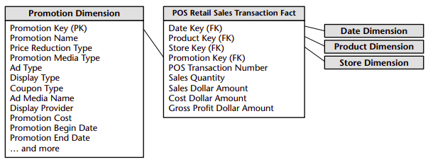
From a purely logical point of view, we could record very similar information about the promotions by separating the four major causal mechanisms (price reductions, ads, displays, and coupons) into four separate dimensions rather than combining them into one dimension. Ultimately, this choice is the designer’s prerogative. We will need to include a row in the promotion dimension, with its own unique key, to identify “No Promotion in Effect” and avoid a null promotion key in the fact table.
Factless table?
Regardless of the handling of the promotion dimension, there is one important question that cannot be answered by our retail sales schema: What products were on promotion but did not sell? In the relational world, a second promotion coverage or event fact table is needed to help answer the question concerning what didn’t happen. The promotion coverage fact table keys would be date, product, store, and promotion in our case study. This obviously looks similar to the sales fact table we just designed; however, the grain would be significantly different. In the case of the promotion coverage fact table, we’d load one row in the fact table for each product on promotion in a store each day (or week, since many retail promotions are a week in duration) regardless of whether the product sold or not. The coverage fact table allows us to see the relationship between the keys as defined by a promotion, independent of other events, such as actual product sales. We refer to it as a factless fact table because it has no measurement metrics; it merely captures the relationship between the involved keys.
(market basket stuffs)
ETL Book
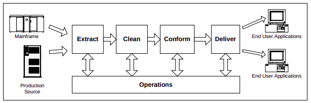
A properly designed ETL system extracts data from the source systems, enforces data quality and consistency standards, conforms data so that separate sources can be used together, and finally delivers data in a presentation-ready format so that application developers can build applications and end users can make decisions.
Two simultaneous threads must be kept in mind when building an ETL system:
- the Planning and Design thread
- the Data Flow thread
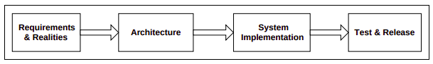
Requirements, Realities and Architecture
Implementation and Operations
From the data warehouse point of view, the ETL marketplace has three categories:
- mainline ETL tool,
- data profiling,
- data cleansing