into Research stuffs

RDS instance:
- Aba RDS instance ta pailai dekhi xa teslai chai usle connect garxa ani locally engine bata run garira hunxa
Redshift cluster:
- To launch the Redshift cluster, you click the ‘Get stsarted with Redshift’.
- The AWS Redshift serverless experience makes it easy for customers to run and scale analytics without having to provision and manage their data warehouse. Simpy load and query data.
- With a few clicks, you can create your first AWS provisioned cluster in minutes
- Fields are:
  - Cluster identifier
  - Can also do free trial for a limited time if your organization has never created Redshift
  - Choose a node type that meets your CPU, RAM, storage capacity, and drive type requirements
  - Can load sample data for test
  - Choose IAM roles??
  - Can customize Network, Security, Backup, Configuration, Maintenance
What is serverless? - it means that you are not responsible for managing and

(I mean jasari RDS lai locally acess garyo ni tesari nai redshift lai ni garxa hola)
- Use the query editor v2 to run queries in your Redshift cluster
- Work with your client tools: You can connect to Redshift from your client tools, such as SQL clients, BI tools, and ETL tools, using JDBC or ODBC drivers. choose cluster and copy JDBC or ODBC URL
- Choose your JDBC or ODB drivers: Use JDBC or ODB drivers to connect to Redshift from your client tools such as SQL clients, BI tools, and ETL tools. We recommend using the new Redshift specific deriver for better performance and scalability.
AWS Glue: (or alternative AWS database migration service (DMS))
- Make connection to RDS and Redshift
- Then he uses the crawler: a crawler connects to a data store, progresses through a prioritized list of classifiers to determine the schema for your data, and then creaets metadata tables in your data catalog.
- he makes two crawlers and these crawlers get the metadata from RDS and Redshift under two databases for each redshift and rds
- Then create a job, like whether to change the schema, perform joins
AWS DMS:
- Make a replication instance
- Do the source and target endpoints
AWS Data Pipeline:
- Highly customizable and work arounds, unoptimized and serial
Open source alternative: Apache airflow
- Install the airflow locally, (or cloud ma ni hunxa hola)
- Then set up the connections
- Some more configurations and scripting to do
Snowflake:
- Separates storage and compute, allowing for dynamic scaling of compute resources. This means you can scale up computing power for demanding queries without impacting other operations.
- Snowflake supports multi cluster configurations for its virtual warehouses enabling it to handle high concurrency
- Can use AWL Glue as well. Wide range of ETL tool intergrations, including native connectors and third-party services like Fivetran, Matillion and Talend
Apache Hive:
- Hive operates on top of Hadoop’s HDFS, organizes data into tables when it uses SQL like language
- Hive queries are executed via MapReduce, Tez or Spart, which can be slower than Redshift’s columnar storage-based queries for certain analytical workloads.
- Hive is not fully manager. Deploying Hive requires setting up and managing Hadoop clusters, either manually or cloud services like EMR (Elsatic MapRedue) which can simplify some aspects of deployment but still requires effort
- Hive is free, but cost for underlyling infrastructure
Presto:
- A distributed SQL query engine designed for interactive analytics and supports quering data from multiple sources
- Comparison based on the type of workloads.

into DuckDB now:

One size fits all? or not? an idea whose time has come and gone:

Relational DBMSs arrived on the scene as research prototypes in 1970’s in the form of System R and INGRES. The main thrust of both prototypes was to surpass IMS in value to customers on the applications that IMS was used for, namely “business data processing”. Hence, both systems were architected for OLTP applications.
Other vendors (Sybase, Oracle, and Informix) followed the same basic DBMS model, which stores relational tables row-by-row, uses B-trees for indexing, uses a cost-based optimizer, and provides ACID transaction properties.
A single code line for all DBMS services means that the database management system (DBMS) uses the same core source code or software base to provide a wide range of database services and functionalities\
The use of multiple code lines causes various practical problems: a cost problem, a compatibility problem, a sales problem, and a marketing problem.
The single code-line strategy has failed due to some key characteristics of data warehouse market.

Points on which databases can diffier : - transactions vs analytics processing - inbound vs outbound (pull or push) - integration (embedded or what?) - synchronization (ACID or otherwise) - availability (recovery methods)

(yesto hunxa bhanni xaina ki yesto chai need ho bhaneko hai, huna ta j ni hunxa sakxa ni lmao)

Analytics vs DBMS

Aspect	OLTP Systems (Traditional DBMS)	OLAP/Data Warehouses
Purpose	Transaction processing, updates.	Business intelligence, complex queries.
Schema	Normalized for transaction efficiency.	Star schema with fact and dimension tables.
Indexes	Prefers B-tree indexes.	Prefers bit-map indexes.
Views	Uses normal (virtual) views.	Uses materialized views.
Data Collection	Direct operation, real-time data handling.	Scraped periodically from operational systems.
Optimization	Optimized for frequent, short transactions.	Optimized for ad-hoc queries.
Storage Model	Row-store, write-optimized: Attributes of a record are stored contiguously, enhancing write performance.	Column-store, read-optimized: Attributes for all rows stored contiguously, enhancing read performance for large, ad-hoc queries.
Data Handling	Designed for efficient handling of a large number of small transactions.	Designed for efficient querying of large amounts of historical data.
Query Performance	Optimized for quick, transactional queries affecting few records at a time.	Optimized for complex queries scanning large datasets, often involving aggregation.
Data Volume	Handles real-time transaction data.	Handles large volumes of historical data.
Compression	Less emphasis on compression due to the transactional nature and need for immediate access.	More effective compression, benefiting from columnar storage and the uniformity of data within each column.
Null Value Handling	Handles null values within the context of row storage, potentially less efficiently.	More efficiently manages null values due to columnar storage, reducing storage space for sparse datasets.

Optimized for star schema type warehousing: snowflake, redshift, bigquery and so on

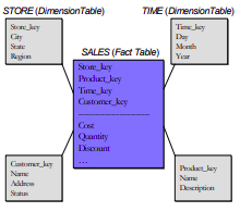
To a first approximation, most vendors have a warehouse DBMS (bit-map indexes, materialized, star schemas, and optimizer tactics for star schema queries) and an OLTP DBMS (B-tree indexes and a standard cost-based optimizer) which are united by a common parser.

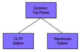
Although this configuration allows such a vendor to market his DBMS product as a single system, because of the single user interface, in effect, she is selling multiple systems.

Inbound processing vs DBMS

Feature	Outbound Processing (Traditional DBMS)	Inbound Processing (Stream Processing)
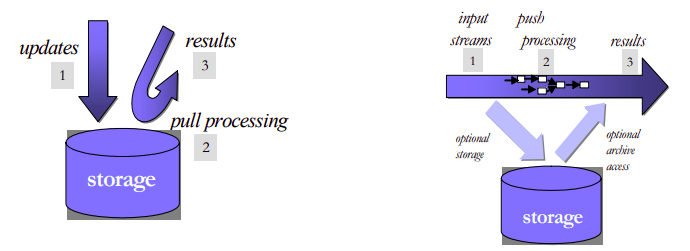
Data Flow	Data is stored first, then processed. (“Process-after-store”)	Data is processed in real-time as it arrives, before optional storage.
Primary Use	Data storage, batch processing, historical data analysis.	Real-time analytics, monitoring, event processing.
Latency	Higher due to the storage step before processing.	Lower, as data is processed on-the-fly without waiting for storage.
Processing Model	Pull model: System pulls data from storage to process queries.	Push model: Incoming data is pushed through queries for immediate processing.
Data Handling	Designed to accept and securely store data, ensuring data persistence.	Focuses on fast, real-time data processing with optional data persistence.
Storage Requirement	Mandatory, as data must be stored before processing.	Optional, can be asynchronous or bypassed entirely for certain use cases.
Query Execution	Executes queries against stored data.	Stores queries and processes incoming data through them.
Examples	Oracle, MySQL, PostgreSQL.	Aurora, StreamBase.
Engine Design	Originally designed for storage then query processing, with later additions like triggers for limited real-time capabilities.	Designed from the ground up for real-time data processing and streaming analytics.
Aggregation	Supports aggregations over static datasets with SQL, useful for batch analysis.	Extends SQL with time windows for aggregations over continuous, unbounded streams.

Traditional vs Embedded

Aspect	Client-server (Traditional DBMS)	Embedded Systems
Space	Separate application and DBMS spaces.	Single integrated space.
Security	Designed for untrusted clients, strict isolation.	Trust within development team, less isolation.
Performance	Process switches add overhead.	No process switches, better performance.
Integration	Limited, uses stored procedures/blades.	Flexible, integrates custom functions and DBMS logic.
State Management	Complex, separate management.	Simplified, within same space.
Use Case	Security/isolation critical.	Real-time, performance critical.
Programming Model	Rigid, clear client-DBMS distinction.	Flexible, mixed logic integration.

Disadvantages of embedded dbms: - a heavy query in sqlite can slow down the entire web server’s response time - SQLite locks the database file during write operations which can limit concurrency - if a web app grows, adding more users might degrade performance since sqlite on the same server limits how much you can scale; - if a web server is compromised, the embedded database is directly at risk

Synchronization

Traditional DBMSs use ACID transactions to provide isolation between concurrent transactions submitted by multiple users. In streaming systems, which are not multi-user, such isolation can be effectively achieved through simple critical sections, which can be implemented through light-weight semaphores. Since full-fledged transactions are not required, there is no need to use heavy-weight locking-based mechanism anymore. In summary, ACID properties are not required in most stream processing applications, and simpler, specialized performance constructs can be used to advantage

High availability

Traditional DBMS log-based recovery mechanisms, designed to ensure precise data and state recovery, may lead to seconds to minutes of downtime, potentially causing data loss if incoming streams aren’t buffered. This recovery approach, while aiming for exact pre-failure state restoration, can introduce significant performance overhead. It’s most suitable for applications demanding strict data integrity. On the other hand, alternative high availability techniques, such as using “hot standby” machines, aim to minimize downtime and reduce the risk of data loss by maintaining continuous operation, often foregoing logging to lessen performance impact. These methods may allow for some data loss or duplication, making them more fitting for real-time or streaming applications where brief inaccuracies are tolerable and the focus is on maintaining broader application state beyond just tabular data.

Specific types of databases

Data warehouses:
Sensor networks
Text search (elastic search):
Scientific databases:
XML databases:

DuckDB specifics

From docs:

Snowflake is a platform, while DuckDB is a database engine

in terms of github stars, duckdb = postgres

Benefits: - In process, runs everywhere, as a python library - Jupyter, CI, Cloud etc. - Even runs in your browser (WASM), there is a QR, you scan and run DuckDB in browser of phone - Flexible extension mechanism: reads JSON, Parquet, directly from S3 - Endless integration possibilities - DuckDB is just a binary, no credentials, ACL, firewalls, etc. - No dependencies. - Dataframes: In Python library can query and store results in pandas.DataFrame(s) - pandas + DuckDB = wow - Works hard to avoid OOMs (offloads to disk as needed) - Simplicity wins at the long run

Syntactic queries (DuckDB SQL deviation from ANSI SQL): - GROUP BY ALL - SELECT * EXCLUDE - ASOF JOIN

Making difference on above points:

Warehouse type (columnar style)
Outbound meaning pull specifics
Embedded
Lightweight ACID implementation
Write-ahead logging

From original paper:

The immense popularity of SQLite shows that there is need for unobtrusive in-process data management solutions. However, there is no such system yet geared towards analytical workloads.

Okay I will review SQLite:

SQLite is a software library that translates high-level disk I/O requests generated by an application into low-level I/O operations that can be carried out by the OS. The application constructs high-level I/O requests using the SQL language. SQLite translates each high-level SQL statement into a sequence of many low-level I/O requests (open a file, read a few bytes from a file, write a few bytes into a file etc.) that do the work requested by the SQL.
An app could do all its disk I/O by direct calls to operating system I/O routines but there are advantages to using a higher level interface based on the SQL language:
1. A few lines of SQL can replace hundreds or thousands of lines of procedural code.
2. SQL and SQLite are transactional.
3. SQLite is often faster than direct low-level I/O.
SQLite is different from most other sql databases:
1. SQLite is server-less software library, whereas the other systems are client-server based. With MySQL, PostgreSQL, SQL-Server, and others, the application sends a message containing some SQL over to a separate server thread or process. That separate thread or process performs the requested I/O, then send the results back to the application. But there is no separate thread or process with SQLite. SQLite runs in the same address space as the application, using the same program counter and heap storage. SQLite does no interprocess communication (IPC). When an application sends an SQL statement into SQLite (by invoking a the appropriate SQLite library subroutine), SQLite interprets the SQL in the same thread as the caller. When an SQLite API routine returns, it does not leave behind any background tasks that run separately from the application.
2. An SQLite database is a single ordinary file on disk (with well-defined file format). With other systems, a “database” is usually a large number of separate files hidden away in obscure directories of the filesystem, or even spread across multiple machines. But with SQLite, a complete database is just an ordinary disk file.

SQL is a programming language: The best way to understand how SQL database engines work is to think of SQL as a programming language, not as a query language. Each SQL statement is a separate program. Applications construct SQL program source files and send them to the database engine. The database engine compiles the SQL source code into executable form, runs that executable, then sends the result back to the application.

Back to DuckDB:

SQL strongly focuses on OLTP workloads, and contains a row-major execution engine operating on a B-Tree storage format. As a consequence, SQLite’s performance on OLAP workloads is very poor.

The following requirements for embedded analytics databases were identified (from their research MonetDBLite):

High efficiency for OLAP workloads, but without completely sacrificing OLTP performance. For example, concurrent data modification is a common use case in dashboard-scenarios where multiple threads update the data using OLTP queries and other threads run the OLAP queries that drive visualizations simultaneously.
Efficient transfer of tables to and from the database is essential. Since both database and application run in the same process and thus address space, there is a unique opportunity for efficient data sharing which needs to be exploited.
High degree of stability, if the embedded database crashes, for example due to an out-of-memory situation, it takes the host down with it. This can never happen.
Practical “embeddability” and portability, the database needs to run in whatever environment the host does.

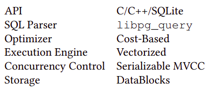
Design and implementation:

Overall, we follow the “textbook” separation of components:

Parser,
logical planner,
optimizer,
physical planner,
execution engine. Orthogonal components are the transaction and storage managers.

Comparison to ClickHouse

Feature/Aspect	DuckDB	ClickHouse
Scalability	Primarily designed for single-node use, optimizing local/single-machine performance.	Horizontally scalable, supports distributed query processing and parallel execution across multiple nodes.
Use Cases	Ideal for local analytics, embedded analytics within applications, and as a tool that leverages cloud resources when necessary.	Suited for real-time analytics, big data processing, event logging, monitoring, IoT, and data warehousing on a large scale.
Database Feel	Feels more like a local, embedded tool optimized for analytics.	Feels like a more full-featured, enterprise-scale database system.
Performance	Optimized for analytical workloads on single-node machines with impressive performance and pain-free setup.	Demonstrates superior performance in scenarios like querying over two billion rows, being 3X faster than DuckDB in some cases.
Runtime Model	Simple and straightforward, ideal for embedded use and local analytics.	More complex due to its capabilities for distributed processing and horizontal scaling.
Innovations and Integrations	Integration with Apache Arrow enhances its capabilities for in-memory analytics. MotherDuck introduces a serverless cloud version.	Offers a lightweight client (`clickhouse-local`) for querying data files directly, expanding its use case scenarios.
Deployment	Low deployment effort, embeddable like SQLite, and optimized for analytics with minimal setup required.	Heavier than DuckDB, primarily operates in server-client mode but also provides a client-only mode for flexibility.
Comparison Remarks	Often compared to a “mutant offspring of SQLite and Redshift,” highlighting its unique position for analytical tasks on single-node machines.	While heavier and more complex, it’s designed for PB-scale data volumes and distributed deployments, offering flexibility in data querying methods.
Community and Development	Growing interest and development around local and cloud-based solutions, with significant contributions like MotherDuck.	Continuously evolving with a focus on enhancing its distributed and real-time processing capabilities for large-scale analytics.

Clickhouse vs Redshift:

Feature/Aspect	Amazon Redshift	ClickHouse
Deployment and Management	Fully managed, cloud-native service offered by AWS. Automated maintenance tasks like backups and scaling.	Open-source and can be self-hosted or cloud-deployed. Manual setup and management, unless using managed services.
Performance and Scalability	Utilizes columnar storage and optimized for complex queries. Managed scaling of storage and compute resources.	High performance on large datasets, especially for real-time analytics. Horizontally scalable with efficient query distribution.
Query Execution	Supports SQL with analytics extensions. Offers materialized views, result caching, and query optimization.	Uses a SQL dialect optimized for real-time analytics. Known for fast query execution on log analysis and time-series data.
Ecosystem and Integrations	Tight integration with AWS services for seamless data workflows. Extensive support for data loading and ETL.	Robust community support with a range of tools for data ingestion and visualization. More manual integration with cloud services.
Cost	Pricing based on cluster size and node types. Offers on-demand and reserved instance pricing models.	Cost-effective for self-managed setups; cloud hosting costs depend on the provider. Open-source nature eliminates licensing fees.

DUCK DB STUFFS

Access MySQL from DuckDB:

pip3 install duckdb

duckdb.execute('INSTALL mysql;')
 
duckdb.execute('LOAD mysql;')
 
duckdb.execute("ATTACH 'host=127.0.0.1 
			user=root 
			password=mk 
			port=3306 
			database=classicmodels' AS mysqldb (TYPE mysql)")
 
duckdb.execute('USE mysqldb;')

DLT and DBT from MySQL to DuckDB:

dlt is an open-source library that you can add to your Python scripts to load data from various and often messy data sources into well-structured, live datasets.

pip3 install dlt

Unlike other solutions, with dlt, there’s no need to use any backends or containers. Simply import dlt in a Python file or a Jupyter Notebook cell, and create a pipeline to load into any of the supported destinations. You can load data from any sources that produces Python data structures, including APIs, files, databases, and more.

Resource:

A resource is a optionally async function that yields data. To create a resource, we add the @dlt.resource decorator to that function.

Commonly used arguments:

name The name of the table generated by this resource. Defaults to decorated function name
table_name the name of the table, if different from resource name.
write_disposition How should the data be loaded at destination? Currently, supported: append, replace and merge. Defaults to append
primary_key define name of the columns that will receive hints.
columns let’s you define one or more columns, including the data types, nullability and other hints.

The 3 write dispositions:

Append: appends the new data to the destination
Full load: replaces the destination dataset with whatever the source produced on this run.
Merge: merges new data to the destination using merge_key and/or de-duplicates or upserts new data using primary_key

Define schema with pydantic:

class User(BaseModel):
	id: int
	name: str
	address: str

Resource:

@dlt.resource(
	name='test',
	table_name="my_table",
	write_disposition='replace',
	primary_key='id',
	columns=User,
)
def generate_rows():  
	for i in range(10):  
		yield {'id':i, 'name':f'Ram{i}', 'address':f'Ktm{i}'}

Dispatch data to many tables: You can load data to many tables from a single resource. The most common case is a stream of events of different types, each with different data schemas. To deal with this, you can use table_name argument on dlt.resource. You could pass the table name as a function with the data item as an argument and the table_name string as a return value.

@dlt.resource(table_name=lambda event: event['type'])

To see the schema of the resource:

generate_rows().compute_table_schema()

{
	'name': 'test', 
	'columns': 
	{
		'id': 
		{
			'name': 'id', 
			'data_type': 'bigint', 
			'nullable': False, 
			'primary_key': True
		}, 
		'name': 
		{
			'name': 'name', 'data_type': 'text', 'nullable': False
		},
	}, 
	'write_disposition': 'merge', 
	'schema_contract':
	{
		'tables': 'evolve', 'columns': 'discard_value', 'data_type': 'freeze'
	}, 
	'resource': 'test'
}

Source:

A source is a logical grouping of resources i.e. endpoints of a single API. The most common approach is to define it in a separate Python module. A source is a function decorated with @dlt.source that returns one or more resources. A source can optionally define a schema with tables, columns, performance hints and more.

@dlt.source
def daily_report_json():
	endpoints = ["key1", "key2", "keyn"]
	
	def get_resource(endpoint):
		for t in daily_report[endpoint]:
			yield t
			
	for endpoint in endpoints:
		yield dlt.resource(get_resource(endpoint), name=endpoint)

The schema describes the structure of normalized data (e.g. tables, columns, data types, etc.) and provides instructions on how the data should be processed and loaded. dlt generates schemas from the data during normalization process. user can affect this standard behavior by providing hints that change how tables, columns and other metadata is generated and how the data is loaded. Such hints can be passed in the code ie. to dlt.resource decorator or pipeline.run method. Schemas can be also exported and imported as files, which can be directly modified.

Attaching schemas to sources:

The dlt.source decorator accepts a schema instance that you can create yourself and modify in whatever way you wish. The decorator also support a few typical use cases. If no schema instance is passed, the decorator creates a schema with the name set to source name and all the settings to default.

If no schema instance is passed, and a file with a name {source name}_schema.yml exists in the same folder as the module with the decorated function, it will be automatically loaded and used as the schema.

We recommend to not create schemas explicitly. Instead, user should provide a few global schema settings and then let the table and column schemas to be generated from the resource hints and the data itself.

Adjust a schema:

Schema is modified in the source function body

Pipeline:

A pipeline is a connection that moves the data from your Python code to a destination. The pipeline accepts dlt sources or resources as well as generators, lists and any iterables. Once the pipeline runs, all resources get evaluated and the data is loaded at destination.

You instantiate a pipeline by calling dlt.pipeline function with following arguments:

pipeline_name a name of the pipeline that will be sued to identify it in trace and monitoring events and to restore its state and data schemas on subsequent runs. If not provided, dlt will create pipeline name from the file name of currently executing Python module.
destination a name of the destination to which dlt will load the data.
dataset_name a name of the dataset to which the data will be loaded. A dataset is a logical group of tables. i.e a schema in relational databases or folder grouping many files.
progress supports 4 progress monitors out of box.

pipeline = dlt.pipeline(
	pipeline_name="tutorial", destination="duckdb", dataset_name="test",
	progress = 'tqdm'
)

To load the data you can call the run method and pass your data in data argument.

data (the first argument) may be a dlt source, resource, generator function, or iterables.
write_disposition controls how to write data to a table. Defaults to append.
- append will always add new data to the end of the table
- replace will replace existing data with new data
- skip will prevent data from loading
- merge will deduplicate and merge based on primary_key and merge_key hints
table_name specified in case when the table name cannot be inferred i.e. from the resources or name of the generator function.

pipeline.run(generate_rows)
 
pipeline.run(source.with_resources("key1", "keyn"))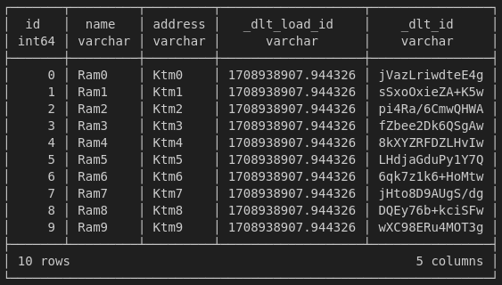

if data is a JSON specifics:

a list of dictionary → a table
a dictionary of list of dictionary → multiple spawn tables

Each resource in your pipeline definition is represented by a table in the destination. When creating a database schema, dlt recursively unpacks nested structures into relational tables, creating and linking children and parent tables.

This is how it works:

Each row in all (top level and child) data tables created by dlt contains UNIQUE column named _dlt_id
Each child table contains FOREIGN KEY column _dlt_parent_id linking to a particular row (_dlt_id1) of a parent table.
Row in child tables come from the lists: dlt stores the position item in the list in _dlt_list_idx.
For tables that are loaded with the merge write disposition, we add a ROOT KEY columns _dlt_root_id, which links child table to a row in top level table.

Staging dataset:

So far we’ve been using the append (or replace) write disposition in our example pipeline. This means that each time we run the pipeline, the data is appended to the existing tables. When you use merge write disposition, dlt creates a staging database schema for staging data. The schema is named <dataset_name>_staging and contains the same tables as the destination schema. When you run the pipeline, the data from the staging tables is loaded into the destination tables in a single atomic transaction.

State:

The pipeline state is a Python dictionary (by default) which lives alongside your data; you can store values in it and, on next pipeline run, request them back. You read and write the state in your resources. Below is an archives which we use to prevent requesting duplicates.

@dlt.resource(
	name='test',
	table_name="my_table",
	write_disposition='replace',
	primary_key='id',
	columns=User,
)
def generate_rows():  
	checked_archives = dlt.current.resource_state().setdefault("archives", [])
	for i in range(10):  
		if i in checked_archives:
			print("Skip")
		else:
			checked_archives.append(i)
			yield {'id':i, 'name':f'Ram{i}', 'address':f'Ktm{i}'}

dlt uses the state internally to implement last value incremental loading. This use case should cover around 90% of your needs to use the pipeline state. If not:

Store a list of already requested entities if the list is not much bigger than 100k elements.
Store large dictionary of last values if you are not able to implement it with the standard incremental construct.

Do not use dlt state when it may grow to millions of elements. Do you plan to store modification timestamps of all of your millions of user records? This is probably a bad idea!

Incremental loading:

Incremental loading is the act of loading only new or changed data and not old records that we already loaded. It enables low-latency low cost data transfer.

The write disposition you choose depends on the data set and how you extract it. To find the write disposition you should use, the first question you should ask yourself is whether my data stateful or stateless? Stateful data has a state that is subject to change - for example a user’s profile. Stateless data cannot change - for example, a recorded event, such as a page view.

Because stateless data does not need to be updated, we can just append it.

For stateful data, comes a second question - Can I extract it incrementally from the source? If not, then we need to replace the entire data set. If however we can request the data incrementally such as “all users added or modified since yesterday” then we can simply apply changes to our existing dataset with the merge write disposition.

DBT-core

Adapters are an essential component of dbt. At their most basic level, they are how dbt connects with the various supported data platforms. At a higher-level, dbt Core adapters strive to give analytics engineers more transferrable skills as well as standardize how analytics projects are structured. Gone are the days where you have to learn a new language or flavor of SQL when you move to a new job that has a different data platform. That is the power of adapters in dbt Core.

There’s a lot more there than just SQL as a language. Databases (and data warehouses) are so popular because you can abstract away a great deal of the complexity from your brain to the database itself. This enables you to focus more on the data:

SQL API
Client library/driver
Server connection manager
Query parser
Query optimizer
Runtime
Storage access layer
Storage

What needs to be adapted?

dbt adapters are responsible for adapting dbt’s standard functionality to a particular database. The outermost layers of a database map roughly to the areas in which the dbt adapter framework encapsulates interdatabase differences. Even amongst ANSI-compliant databases, there are differences in the SQL grammar.

About dbt projects:

A dbt project informs dbt about the context of your project and how to transform your data. By design, dbt enforces the top-level structure of a dbt project such as the dbt_project.yml file, the models directory, the snapshots directory, and so on. Within the directories of the top-level, you can organize your project in any way that meets the needs of your organization and data pipeline.

…

About dbt models:

dbt Core and Cloud are composed of different moving parts working harmoniously. All of them are important to what dbt does — transforming data—the ‘T’ in ELT. When you execute dbt run, you are running a model that will transform your data without that data ever leaving your warehouse.

Models are where your developers spend most of their time within a dbt environment. Models are primarily written as a select statement and saved as a .sql file. While the definition is straightforward, the complexity of the execution will vary from environment to environment. Models will be written and rewritten as needs evolve and your organization finds new ways to maximize efficiency.

Each .sql file contains one model/ select statement.
The model name is inherited from the filename.
Models can be nested in subdirectories within the models directory.

When you execute the dbt run command, dbt will build this model data warehouse by wrapping it in a create view as or create table as statement. By default dbt will:

Create models as views
Build models in a target schema you define
Use your file name as the view or table name in the database

Configuring models:

Configurations are model settings that can be set in your dbt_project.yml file, and in your model file using config block. Some example configurations include:

Changing the materialization that a model uses - a materialization determines the SQL that dbt uses to create the model in your warehouse.
Build the models into separate schemas.
Apply tags to a model.

My Knowledge Base

Explorer

GZ Research into DuckDB and DBT