Unsupervised Learning

Autoencoders

The goal of deep learning involves building a probabilistic model of the input, $p_{\text{model}}(x)$. Such a model can, in principle, use probabilistic inference to predict any of the variables in its environment given any of the other variables. Many of these models also have latent variables $h$, with $p_{\text{model}}(x)=E_h{p}_{\text{model}}(x|h)$. These latent variables provide another means of representing the data.

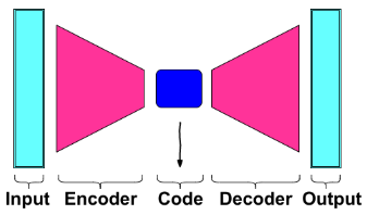
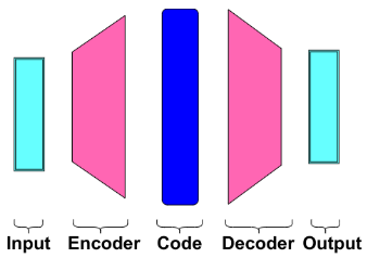
An autoencoder is a neural network that is trained to attempt to copy its input to its output. Internally, it has a hidden layer $h$ that describes a code used to represent the input. The network may be viewed as consisting of two parts: an encoder function $h=f(x)$ and a decoder that produces a reconstruction $r=g(h)$. If an autoencoder succeeds in simply learning to set $g(f(x))=x$ everywhere, then it is not especially useful. Instead, autoencoders are designed to be unable to learn to copy perfectly.

Usually, they are restricted in ways that allows them to copy only approximately, and to copy only input that resembles the training data. Because the model is forced to prioritize which aspects of the input should be copied, it often learns useful properties of the data.

Undercomplete:

Overcomplete: (denoising)

Since the autoencoder learns the identity function, we are facing the risk of overfitting when there are more network parameters than the number of data points. To avoid overfitting and improve the robustness, Denoising autoencoder proposed a modification to partially corrupt the input by adding noises to or masking some values of the input vector in stochastic manner. Then the model is trained to recover the original input not the corrupt one.

A denoising autoencoder (DAE) minimizes $L(x,g(f(\tilde{x})))$, where $\tilde{x}$ is a copy of $x$ that has been corrupted by some form of noise. Denoising autoencoders must therefore undo this corruption rather than simply copying their input. Denoising training forces $f$ and $g$ to implicitly learn the structure of $p_{\text{data}}(x)$. They provide an example of how useful properties can emerge as a byproduct of minimizing the reconstruction error. They are also an example of how over complete, high-capacity models may be used as autoencoders as long as care is taken to prevent them from learning the identity function.

We introduce a corruption process $C(\tilde{x}|x)$, which represents a conditional distribution over corrupted samples $\tilde{x}$, given a data sample $x$. The autoencoder then learns a reconstruction $p_{\text{reconstruct}}(x|\tilde{x})$ estimated from the training as $p_{\text{decoder}}(x|h)$ with $h$ the output of encoder $f(\tilde{x})$ and $p_{\text{decoder}}$ typically defined by a decoder $g(h)$. We can therefore view the DAE as performing stochastic gradient descent on the following expectation: $-E_{x\sim {\hat{p}}_{\text{data}}(x)}{E}_{\tilde{x}\sim C(\tilde{x}|x)}\log p_{\text{decoder}}(x|h=f(\tilde{x}))$

Score matching is an alternative to maximum likelihood. It provides a consistent estimator of probability distributions based on encouraging the model to have the same score as the data distribution at every training point $x$. In this context, the score is a particular gradient field: ${\nabla }_x\log p(x)$ The gradient field of $\log p_{\text{data}}$ is one way to learn about the structure of $p_{\text{data}}$ itself. When the denoising autoencoder is trained to minimize the average of squared errors $||g(f(\tilde{x}))-x|{|}^2$, the reconstruction of $g(f(\tilde{x}))$ estimates $E_{x,\tilde{x}\sim p_{\text{data}}(x)C(\tilde{x}|x)}[x|\tilde{x}]$. The vector $g(f(\tilde{x}))-x$ points approximately estimates the score ${\nabla }_x\log p_{\text{data}}(x)$ up to a multiplicative factor that is the average root mean square reconstruction error.

Structured probabilistic models

VAE:

The generative models are about producing more examples that are like those already in the dataset but not exactly the same. They could start with a database of raw images and synthesize new, unseen images. The complicated dependencies between the dimensions make the models more difficult to train.

The goal is to train a model to generate new samples from a probability distribution $p_{\text{model}}(x)$, such that these generated samples are similar to those from $p_{\text{data}}$ the true data distribution:

VAE:

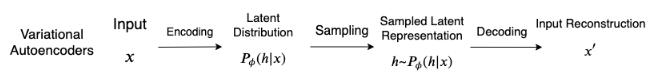
Variational auto-encoders are associated to autoencoders of its architectural affinity but are significantly different in the goal and mathematical formulation. Instead of encoding the data as a single point over latent space as in autoencoders, VAE encodes the distribution over the latent space which ensures regularized code present in the bottleneck. In a latent variable model, we posit that our observed data $x$ is a realization of another random variable $X$. Moreover, we posit the existence of another random variable $Z$ where $X$ and $Z$ are distributed according to joint distribution $P(X,Z;\theta )$ where $\theta$ parameterizes the distribution. Unfortunately, our data is only a realization of $X$, not $Z$, and therefore $Z$ remains latent.

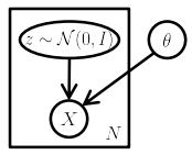
Formally, say we have a vector of latent variables $z$ in high dimensional space $Z$ which we can easily sample according to some probability density function $P(z)$ defined over $Z$. Then, say we have a family of deterministic functions $f(z;\theta )$, parameterized by a vector $\theta$ in some space $\Theta$, where $f:Z\times \Theta \to X$. $f$ is deterministic, but if $z$ is random and $\theta$ is fixed, then $f(z;\theta )$ is a random variable in the space $X$ .

The wish is to optimize $\theta$ such that we can sample $z$ from $P(z)$ and, with high probability, $f(z;\theta )$ will be like the $X$’s in our dataset.

Why $z\sim N(0,1)$?

VAEs assume that there is no simple interpretation of the dimensions of $z$, and instead assert that samples of $z$ can be drawn from a simple distribution, i.e. $N(0,I)$, where, $I$ is the identity matrix. The key is to notice that any distribution in $d$ dimensions can be generated by taking a set of $d$ variables that are normally distribution and mapping them through a sufficiently complicated function.

For example, say we wanted to construct as 2D random variable whose values lie on a ring. If $z$ is 2D and normally distribution, $g(z)=z/10+z/||z|||$ is roughly ring-shaped:

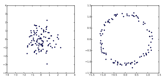
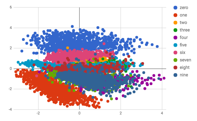
Hence, with powerful function approximators, VAE can simply learn a function which maps independent, normally distributed $z$ values to whatever latent variables might be needed and then map those latent variables to $X$. If $f(z;\theta )$ is a multi-layer neural network, then the network maps the normally distributed $z^{\prime }$s to the latent values with its first few layers then it can use later layers to map those latent values to a fully-rendered digit. If such latent structure helps the model accurately maximize the likelihood of the training set, then the network will learn that structure in some layer:

How to ensure that $P(X)$ is biased for our data?

The mathematical notion is to maximize the probability of each $X$ in the training set under the entire generation process, according to: $P(X)=\int P(X|z;\theta )P(z)dz$. If the latent space representation is a high multi-dimensional space, computing the marginal likelihood requires multi-variable integration which is very complex and intractable.

In practice, for most $z$, $P(X|z)$ will be nearly zero and hence contribute nothing to the estimate of $P(X)$. The key idea behind the variational autoencoder is to attempt to sample values of $z$ that are likely to have produced $X$, and compute $P(X)$ just from those.

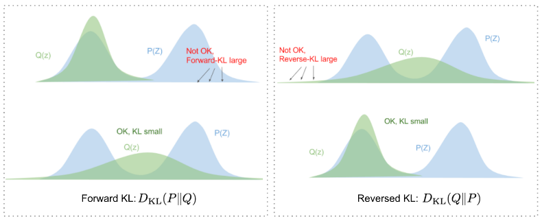
This means we need a new function $Q(z|X)$, the encoder, which take a value of $X$ and gives a distribution over $z$ values that are likely to produce $X$. Our goal is to minimize Kullback-Leibler divergence between $P(z|X)$ and $Q(z|X)$. (But why reverse instead of forward?) $D[Q(z|X)||P(z|X)]=E_{z\sim Q(z|X)}\log \frac{Q(z|X)}{P(z|X)}$ (The KL divergence, also known as relative entropy, measures how much a probability distribution differs from another probability distribution.)

Applying Bayes rule: $D[Q(z|X)||P(z|X)]=E_{z\sim Q}[\log Q(z|X)-\log P(X|z)-\log P(z)]+\log P(X)$ Here, $\log P(X)$ comes out of the expectation because it does not depend on $z$. Negating both sides, rearranging, and contracting part of $E_{z\sim Q}$ into a KL-divergence terms yields:

$\log P(X)-D[Q(z|X)||P(z|X)]=E_{z\sim Q(z|X)}[\log P(X|z)]-D[Q(z|X)||P(z)]$

The left hand side has the quantity we want to maximize: $\log P(X)$ plus an error term, which makes $Q$ produce $z^{\prime }$s that can reproduce a given $X$. We want to maximize the log likelihood of generating real data and also minimize the difference between the real and estimated posterior distributions. The negation of which defines our loss function. In Variational Bayesian methods, this loss function is known as the variational lower bound, or evidence lower bound. The lower bound part in the name comes from the fact that KL divergence is always non-negative and thus is the lower bound of $\log P(X)$.

The right hand side is something we can optimize via stochastic gradient descent given the right choice of $Q$. The right hand side takes a form which looks like an autoencoder, since $Q$ is encoding $X$ into $z$ and $P$ is decoding it to reconstruct $X$.

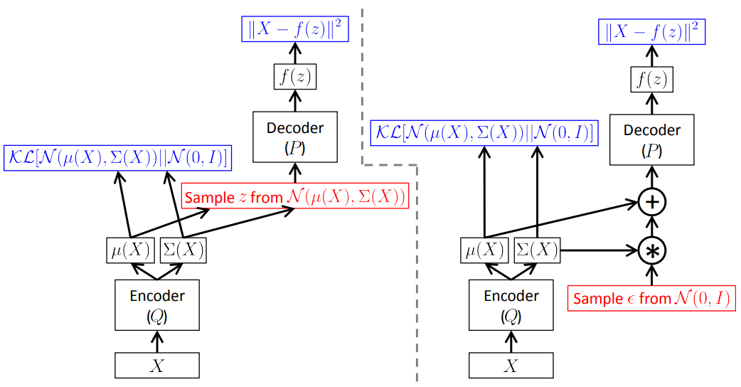
The usual choice is to say that $Q(z|X)=N(z|\mu ,\Sigma )$ where $\mu$ and $\Sigma$ are arbitrary deterministic functions implemented via neural networks. The last term $D[Q(z|X)||P(z)]$ is now a KL-divergence between two multivariate Gaussian distributions, which can be computed in closed form as: $D[N(\mu (X),\Sigma (X))||N(0,1)]=\frac{1}{2}(tr(\Sigma (X))+\mu (X{)}^T\mu (X)-k-\log det(\Sigma (X)))$ where $k$ is the dimensionality of the distribution.

The forward pass works fine and, if the output is averaged over many samples of $X$ and $z,$produces the correct expected value, however, we need to back-propagate the error through a layer that samples $z$ from $Q(z|X)$ which is a non-continuous operation and has no gradient. Parameterization trick here:

Generative adversial networks

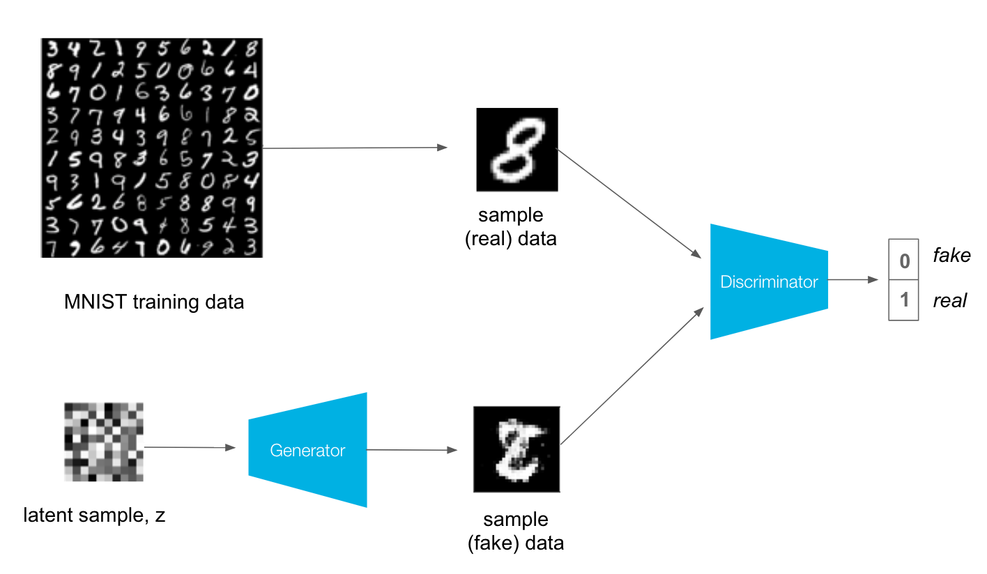
The adversarial nets framework pits the generative model against an adversary: a discriminative model that learns to determine whether a sample is from the model distribution or the data distribution. The generative model can be thought of as analogous to a team of counterfeiters, trying to produce fake currency and use it without detection, while the discriminative model is analogous to the police, trying to detect the counterfeit currency.

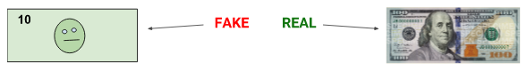
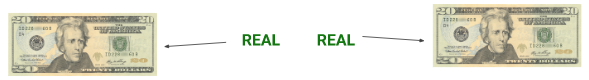
Competition in this game drives both teams to improve their methods until the counterfeits are indistinguishable from the genuine articles. The adversarial modeling framework is most straightforward to apply when the models are both multilayer perceptrons.

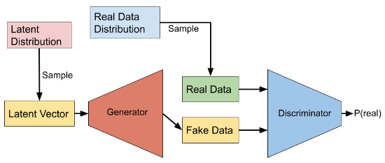
To learnt the generator’s distribution $p_g$ over data $x$, we define a prior on input noise variables $p_z(z)$, then represent a mapping to data space as $G(z;{\theta }_g)$, where $G$ is a differentiable function represented by a multilayer perceptron with parameters ${\theta }_g$.

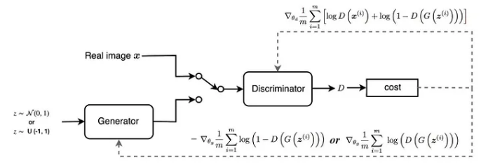
We also define a second multilayer perceptron $D(x;{\theta }_d)$ that outputs a single scalar. $D(x)$ represents the probability that $x$ came from the data rather than $p_g$. We train $D$ to maximize the probability of assigning the correct label to both training examples and samples from $G$. We simultaneously train $G$ to minimize $\log (1-D(G(z))$. In other words, $D$ and $G$ play the following two-player minimax game with value function: ${\text{min}}_G{\text{max}}_{D}V(D,G)=E_{x\sim p_{\text{data}}(x)}[\log D(x)]+E_{z\sim p_z(z)}[\log (1-D(G(z)))]$ Mind explaining? The value function is for the GAN as a whole, which is equivalent to negative cross entropy:

For discriminator: The goal of the discriminator is to correctly classify the given data as real or fake. This can be expressed by the value function as: $V(D)=t\log D(x)+(1-t)\log (1-D(x))$where, $t$ is the target for $D$. $t=0$ for fake samples and $t=1$ for real samples.

If the data is sampled for data $(t=1)$: $V(D{)}_{\text{real}}=\log D(x)$If the data is generated by $G$ given latent vector $z$: $V(D{)}_{\text{fake}}=\log (1-D(G(z)))$ The goal of the training $D$ is to maximize the combined value function: $V(D)=\log (D(x))+\log (1-D(G(z)))$

For generator: The goal of the generator is to fool the discriminator, i.e. to generate data such that $D$ classifies the generated data as real. The value function is written as:$V(G)=t\log D(x_{\text{fake}})+(1-t)\log (1-D(x_{\text{fake}}))$where, $t$ is the target for $D$.

Since the training the generator does not involve real data samples and only fake data with $t=0$, the value function for $G$ simplifies into: $V(G)=\log (1-D(x_{\text{fake}})=\log (1-D(G(z)))$ The goal of $G$ is to minimize this value function $V(G)$.

How to train a GAN? In GAN, the generator and discriminator are trained separately:

Train $D$:

• Sample a mini-batch of $m$ latent vectors $\{z^{(1)},\dots ,z^{(m)}\}$ from latent distribution $p_z(z)$ and utilize which to generate a multi batch of $m$ data samples $\{{\hat{x}}^{(1)},\dots ,{\hat{x}}^{(m)}\}$ from $G$;
• Feed the $m$ samples into $D$ to predict the probabilities $\{{\hat{y}}^{(1)},\dots ,{\hat{y}}^{(m)}\}$;
• Sample a mini batch of $m$ real examples $\{x^{(1)},\dots ,x^{(m)}\}$ from training data distribution;
• Feed the sampled $m$ data into $D$ to predict the probabilities $\{y^{(1)},\dots ,y^{(m)}\}$;
• Update $D$ by performing gradient ascent on the value function: $\frac{1}{m}{\sum }_{i=1}^m[\log y^{(i)}+\log (1-{\hat{y}}^{(i)})]$ Train G:
• Sample a mini-batch of $m$ latent vectors $\{z^{(1)},\dots ,z^{(m)}\}$ from latent distribution $p_z(z)$ and utilize which to generate a multi batch of $m$ data samples $\{{\hat{x}}^{(1)},\dots ,{\hat{x}}^{(m)}\}$ from $G$;
• Feed the $m$ samples into $D$ to predict the probabilities $\{y^{(1)},\dots ,y^{(m)}\}$;
• Update $G$ by performing gradient ascent on the value function: $\frac{1}{m}{\sum }_{i=1}^m\log (1-{\hat{y}}^{(i)})$

The GAN converges when $D$ can no longer discriminate between real and fake data. In this case, ideally one can expect the discriminator output of $\hat{y}=0.5$ for all generated data and real data; the discriminator is only half sure that data is real which also implies that it is half sure that the data can be fake. This is the case when $G$ becomes successful in producing indistinguishable fakes.

The minimax game achieves a global optimum if and only if the probability distribution of $G$ ie $p_g$ matches the real data $p_{\text{data}}$. This is proved in two parts:

As the function $y\to a\log (y)+b\log (1-y)$ achieves its maximum in $[0,1]$ at $\frac{a}{a+b}$ so, for $G$ fixed, the optimal discriminator $D$ is $D_G^{\ast }(x)=\frac{p_{\text{data}}(x)}{p_{\text{data}}(x)+p_g(x)}$ The minimax can now be reformulated as: $C(G)={\text{max}}_{D}V(G,D)=E_{x\sim p_{\text{data}}}\left[\log \frac{p_{\text{data}}(x)}{p_{\text{data}}+p_g(x)}+\right]{+}_{x\sim p_{\text{g}}}\left[\log \frac{p_{\text{g}}(x)}{p_{\text{data}}+p_g(x)}\right]$ For $p_g=p_{\text{data}}$, $C(G)=-\log 4$.

Necessary and sufficient:

The equation can be written in the form of KL divergence terms: $C(G)=-\log 4+KL\left(p_{\text{data}}||\frac{p_{\text{data}}+p_g}{2}\right)+KL\left(p_{\text{g}}||\frac{p_{\text{data}}+p_g}{2}\right)$ The Jenson-Shannon divergence is the distance measure between two probability distribution and is very similar to KL divergence, except that it is symmetric. The JSD is zero only iff the distributions are equal.

Note: If $G$ and $D$ have enough capacity, and at each step, $D$ is allowed to reach its optimum given $G$, and $p_g$ is updated so as to improve the value criterion then $p_g$ converges to $p_{\text{data}}$.

The GAN suffers following major problems:

Discriminator behavior:

The generator cannot learn well if the discriminator is too strong or too weak. Both the models should learn constantly without one being superior to the other for both to improve themselves.

Mode collapse:

When training a GAN, if the generator learns to produce only one type of realistic output (digit 1 in our case), it successfully fools the discriminator. It does not need varying modes and therefore produces same realistic output for all latent vectors. In such case, the discriminator, trying to discriminate the fake and real data, learns to classify all such examples as fake. Hence, the discriminator is stuck at some local minima. The generator in next iterations learns to generate another single type of output to best fool the discriminator. This cycle continues and both the discriminator and generator never learn anything beyond this.

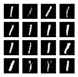
Both of the models are overfitted to exploit the short-term weakness of the opponents rather than optimize for our desired goal to generate all modes similar to training data distribution. This problem of GAN is called as mode collapse.

WGAN??

Hopfield? Boltzmann? SOM?

Diffusion models

Stable diffusion is focused on mathematical way but he focuses on another way

suppose we have a black box API:

image → a black box → probability that it is a handwritten digit

if we have such function we can use it to generate handwritten digit (whatever that means) how?

say the image is 28 x 28 and we change a pixel or so then the probability changes, and we can do it for each and every digit in the image

so what we have done is ${\nabla }_{x}P(\text{image})$ which has 28 x 28 elements there, those values tell us how we can change the pixels to get to handwritten digits

here instead of changing the weights with respect to gradients we are changing the inputs

so we want to train a neural net that tells us which pixel to change to make it more like handwritten

we could create training data: hand written digits + some amount of noise.

but awkward to assign score to images with noise, what to say more noise or less noise?

so instead we measure the amount of measure of noise, he gives example of N(0, std) or, we could predict the exact noise image

our loss? we already have the noise we inputted with our image so just do the MSE there

hence, image = inputted image - predicted noise

so when we pass pure noise its gonna spit out some part thats noisy and leave out some portion that looks like handwritten image so we subtract it from original image (time some constant rey??) then we do it multiple times because pailo choti mai nice aauxa bhanni ta xaina ni

The particular type of neural network is called the unet that inputs somewhat noisy inut and outputs noise

but training such network with inputs of size containing 512 x512 x 3 pixels is damn tight

so instead the unets now take somewhat noisy latents and unnoisae them and the decoder parat decodes to the large image

what about texting the image generator? how do we say it to generate 3 for us

so we will pass (on training unets) the noisy input and also the label of the image so we would guess that its going to be better at getting out the noise, because everything that does not resonantse with given guidance then it is the noise

what about “cute teddy?” we need o convert it into latents that represent it, clip text encoder

they use idea of noise to relate a monotically decreasing function of noise, meaning if t is large then the amont of noise in the image is less

when we find noise we do not directly subtract it, mathi bracket ma halera gareko thiye ni, instead we do mutlily by a constant because our model does nto handle that it only handle latents that are somehow noisy rey

wait this looks like learnin rate so Adam man??

somehow the model also take ‘t’ as input coz the model will do good i u tell it how muc noiseis there

rev: we start with a digit 7 and add some noise, and we present the noisy 7 as an input to an unet to predict the noise, and compares the prediction to the actual noise which is a loss, to make it easy for unet we could pass also an embedding of digit 7

(this skips VAE or latent thingy)

the text and image both go together as: we create embedding for image and also for text and we say to a loss function that these embeddings must look similar. called contrastive loss

so we send embedding + noise to unet and it predicts noise, but it does bad job in the beginning so we subtract it with some constant

he gives example of 54 steps of noise reduction to produce his image, he says early days took around 1000 steps

and he goes on to describe a recently published paper that he says has outdated everything?? that takes 60 steps to 4 steps:

Progressive distillation: is like a common thing you do where there is a trained teacher model that is slow and big which feeds the student model to become faster and do the same job

in diffussion: say step 1 to step 20 which should have taken one step: we train another unet with step 1 input and make it learn to produce step 20 output

there is also a similar paper for guided models

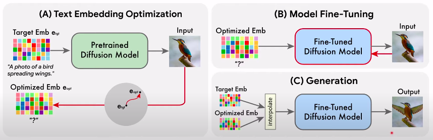
yet another paper: you can pass in image and text and return the edited output,

(dont know this man)

(and there is some jupyter notebook stuff going on)