Python Data

Numpy

NumPy is a successor to the Numeric array object, aiming to establish a foundation for scientific computing. The author, a graduate student in biomedical imaging, discovered Python and Numeric in 1998 and became involved in the Numeric Python community. Pearu Peterson’s development of f2py facilitated wrapping Fortran programs into Python, contributing to scientific computing with Python. In 2001, SciPy was formed through the collaboration of the author, Eric Jones, and Pearu Peterson, combining Python modules for scientific computing. Numarray was created as a replacement for Numeric, leading to some fragmentation in the Python scientific computing community. The author initiated efforts to bring the community together, ultimately resulting in the development of NumPy, released in 2006. NumPy 1.0 was released in late 2006, offering enhanced universal functions and features, and the package adopted the NumPy name.

Sub-package	Purpose	Comments
core	basic objects	all names exported to numpy
lib	additional utilities	all names exported to numpy
linalg	basic linear algebra	old LinearAlgebra from Numeric
fft	discrete Fourier transforms	old FFT from Numeric
random	random number generators	old RandomArray from Numeric
distuils	enhanced build and distribution	improvements built on standard disutils
testing	unit-testing	utility functions useful for testing
f2py	automatic wrapping of Fortan code	a useful utility needed by SciPy

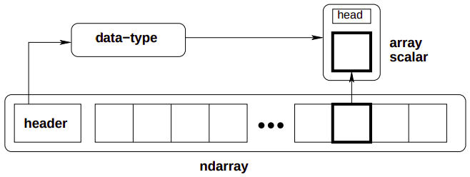
NumPy provides two fundamental objects: an N-dimensional array object (ndarray) and a universal function object (ufunc). An N-dimensional array is a homogeneous collection of items indexed using N integers. There are two essential pieces of information that define an N-dimensional array:

the shape of the array
the kind of item the array is composed of

np.array(object=, dtype=None, copy=True)

An ndarray is an N-dimensional array of items where each item takes up a fixed number of bytes. Typically, this fixed number of bytes represents a number (e.g. integer or floating-point). However, this fixed number of bytes could also represent an arbitrary record made up of any collection of other data types. NumPy achieves this flexibility through the use of a data-type (dtype) object. Every array has an associated dtype object which describes the layout of the array data. Every dtype object, in turn, has an associated Python type-object that determines exactly what type of Python object is returned when an element of the array is accessed.

Memory layout:

Each of these arrays take 12 blocks of memory. How this memory is used to form the abstract 2-dimensional array can vary, however, the ndarray object supports both style.

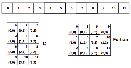
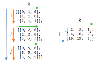
In the C-style of N-dimensional indexing, the last N-dimensional index varies the fastest. In other words, to move through computer memory sequentially, the last index is incremented first, followed by the second-to-last index and so forth. In the Fortran-style of N-dimensional indexing, the first N-dimensional index varies the fastest. Thus, to move through computer memory sequentially, the first index is incremented first until it reaches the limit in that dimension, then the second index is incremented and the first index is reset to zero. The styles of memory layout for arrays are connected through the transpose operation. Thus, if $A$ is a C-style array, then the same block of memory can be used to represent $A^{T}$ as a (contiguous) Fortran-style array.

(arrays are stored as what (C or Fortan) contiguous)

Let $n_{i}$ be the value of the $i$ th index into an array whose shape is represented by the $N$ integers $d_{i} (i = 0 \dots N - 1)$ . The formulas for the one-dimensional index of the N-dimensional arrays reveal what results in an important generalization for memory layout. Note that each formula can be written as: $n^{X} = \sum_{i = 0}^{N - 1} n_{i} s_{i}^{X}$ where $s_{i}^{X}$ gives the stride for dimension $i$ . Thus, for $C$ and Fortan contiguous arrays respectively we have: $s_{i}^{C} = d_{i + 1} d_{i + 2} \dots d_{N - 1}$ $s_{i}^{F} = d_{0} d_{1} \dots d_{i - 1}$ As long as we always use the stride information to move around in the N-dimensional array, we can use any convenient layout we wish for the underlying representation as long as it is regular enough to be defined by constant jumps in each dimension. The ndarray object of NumPy uses this stride information and therefore the underlying memory of an ndarray can be laid out dis-contiguously. An important situation where irregularly strided arrays occur is array indexing.

Universal functions:

The ufunc is an instance of a general class so that function behavior is same. All ufuncs perform element by element operations over an array or a set of arrays (for multi-input functions). An important aspect of ufunc is the idea of broadcasting. Broadcasting allows ufuncs to deal in a meaningful way with inputs that do not have exactly the same shape. In particular,

The first rule of broadcasting is that if all input arrays do not have the same number of dimensions, then a 1 will be prepended to the shapes of the smaller arrays until all the arrays have the same number of dimensions.
The second rule of broadcasting ensures that arrays with a size of 1 along a particular dimension act as if they had the same size of the array with the largest shape along that dimension. The value of the array element is assumed to be the same along that dimension for the broadcasted array.

The most common alternation needed is to route-around the automatic prepending of 1’s to the shape of the array. If it is desired, to add 1’s to the end of the shape, then dimension can be added using np.newaxis name in NumPy.

Application: One important aspect of broadcasting is the calculation of functions on regularly spaced grids. For example, suppose it is desired to show a portion of the multiplication table by computing the function a*b on a grid with a and b running from.

a[:,newaxis]*b

The Array Attributes:

Array attributes reflect information that is intrinsic to the array itself. The exposed attributes are the core parts of an array and only some of them can be reset meaningfully without creating a new array.

Attribute	Description
flags	dictionary-like attributes showing the state of flags in this array
ndim, shape	number of dimensions in array, array shape tuple
size, itemsize, nbytes	number of elements, element size, number of bytes
dtype	data-type object for this array
strides	bytes to jump in the data segment to get from one entry to next

In NumPy, the ndarray object has many methods which operate on or with the array in some fashion, typically returning an array result.

The Array Methods:

The ndarray object has many methods which operate on or with the array in some fashion, typically returning an array result.

Array conversion methods:

Method	Arguments	Description
astype	(dtype {None})	Cast to another data type
copy	()	Copy array
tolist	()	Array as a nested list
dump	(file)	Pickle to stream or file
dumps	()	Gets pickled string

Array shape manipulation:

Method	Arguments	Description
reshape	(newshape, order=‘C’)	Return an array that uses same data but new shape
transpose	()	Return an array view with the shape transposed
flatten	()	Return a new 1-d array with data copied from self
ravel	()	Return a 1-d version of self

Array item selection and manipulation:

Basic indexing:

Indexing is a powerful tool in Python and NumPy takes full advantage of this power. There are three differences:

slicing can be done over multiple dimensions
exactly one ellipsis object can be used to indicate several dimensions at once
slicing cannot be used to expand the size of an array (unlike lists)

There are two kinds of indexing available using X[obj] syntax: basic slicing, and advanced indexing, where X is the array to-be-sliced and obj is the selection object. These two methods of slicing have different behavior and are triggered depending on obj.

Basic slicing occurs when obj is a slice object (constructed by start:stop:step) notation inside of brackets), an integer, or a tuple of slice objects and integers. Ellipsis and newaxis object interspersed with these as well. In Python X[(exp1, exp2, ..., expN)] is equivalent to X[exp1, exp2, ...., expN] as the latter is just syntactic sugar for the former.

The basic slice syntax is i:j:k where $i$ is the starting index, $j$ is the stopping index, and $k$ is the step $(k \neq = 0)$ .
An integer, $i$ , returns same values as i:i+1 except the dimensionality of the returned object is reduced by 1.
You may use slicing to set values in the array, but unlike lists you can never grow the array. The size of the value to be set in X[obj] = value must be broadcastable to the same shape as X[obj].

Advanced selection: ((WHAT THE?))

Advanced selection is triggered when the selection object, obj is

a non-tuple sequence object,
an ndarray (of data type integer or bool), or
a tuple with at least one sequence object or ndarray (of data type integer or bool). There are two types of advanced indexing: integer and Boolean. Advanced selection always returns a copy of the data (contrast with basic slicing that returns a view.)

… The advanced selection occurs when obj is an array object of Boolean type (such as may be returned from comparison operators). The special case when obj.ndim == X.ndim is worth mentioning. In this case, X[obj returns a 1-dimensional array filled with th elements of X corresponding to the True values of obj. The search order will be C-style (last index varies the fastest).

Array object calculation methods:

Many of the methods take an argument named axis. In such cases, if axis is None (the default), the array is treated as a 1-d array and the operation is performed over the entire array. If axis is an integer, then the operation is done over the given axis (for each 1-d subarray that can be created along the given axis). The parameter dtype specifies the data type over which a reduction operation (like summing) should take place.

Method	Arguments	Description
max, min, mean	(axis=None)	maximum/minimum/mean of self
sum, prod	(axis=None)	add/multiply elements of self together
var, std	(axis=None)	variance/standard deviation of self
all, any	(axis=None)	true if all/any entries are true
argmax, argmin	(axis=None)	index of largest/smallest value
clip	(min=, max=)	self[self>max]=max; self[self<min]=min

Basic routines:

Creating arrays:

Routine	Arguments
arange	(start=, stop=None, step=1, dtype=None)
linspace	(start=, stop=, num=50)
zeros	(shape=, dtype=int)
zeros_like	(arr)
ones	(shape=, dtype=int)
ones_like	(arr)
identify	(n, dtype=intp)
where	(condition[, x, y])

where: Returns an array shaped like condition, that has elements of x and y respectively where condition is respectively true or false. If x and y are not given, then returns n-dimensional index for elements of the n-dimensional array self that meet the condition into an n-tuple of equal-length index arrays.

(where prepares for advanced indexing i guess)

Operations on two or more arrays:

Routine	Arguments	Remarks
inner	(a, b)
dot	(a, b)
matmul	(a,b)	(tensor contraction)
outer	(a, b)	A.ravel()[:,newaxis] x B.ravel()[newaxis,:]
convolve	(x, y, mode=‘valid’)	polynomial multiplication for 1-d arrays
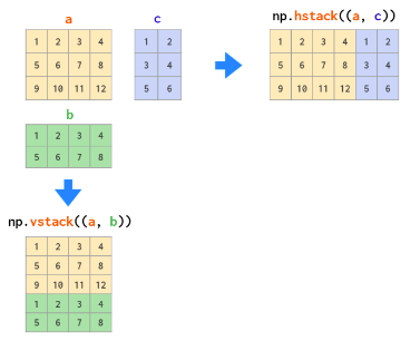
concatenate	(seq=, axis=0)	must have compatible types
vstack	(seq)	stack a sequence of arrays along the first axis
hstack	(seq)	stack a sequence of arrays along the second axis
einsum	(subscripts, *operands)

inner vs dot:

The inner product between two arrays is an array that has shape a.shape[:-1]+b.shape[:-1] with elements computed as the sum of the product of the elements from the last dimensions of a and b. In particular, let I and J be the super indices selecting the 1-dimensional arrays a[I,:] and b[J,:], the the resulting array, r, is: $r [I, J] = \sum_{k} a [I, k] b [J, k]$ Ordinary inner product of vectors for 1-D arrays, in higher dimensions a sum product over the last axes.

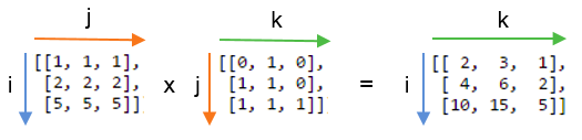
The dot product between two arrays is product-sum over the last dimension of a and the second-to-last dimension of b. Specially, if I and J are super indices for a[I,:] and b[J,:,j] so that j is the index of the last dimension of b. Then shape of the resulting array is a.shape[:-1]+b.shape[:-2]+b.shape[-1] with elements: $r [I, J, j] = \sum_{k} a [I, k] b [J, k, j]$ For 2-D arrays it is equivalent to matrix multiplication, and for 1-D arrays to inner product of vectors. For N dimensions it is a sum product over the last axis of a and the second-to-last axis of b.

hstack vs vstack:

The OG einsum:

Suppose we have two arrays, A and B. Now we want to :

multiply A and B in a particular way to create a new array of products, and then maybe
sum this new array along particular axes, and/or
transpose the axes of the array in a particular order Then there is a good chance einsum will help us do this much faster and more memory-efficiently that combinations of the NumPy functions multiply, sum and transpose would allow.

The key is to choose the correct labelling for the axes of the inputs arrays and the array that we want to get out. A good example to look at is matrix multiplication, which involves multiplying rows with columns and then summing the products. For two 2D arrays A and B, matrix multiplication can be done with:

np.einsum('ij,jk->ik', A, B)

The left-hand part of the labels the axes of the input arrays: ij labels A and jk labels B. The right-hand part of the string labels the axes of the single output array with the letters ik. Drawing on the labels:

Repeating letters between input arrays means that values along those axes will be multiplied together. The products make up the values for the output array.

Omitting a letter from the output means that values along that axis will be summed.

We can return the unsummed axes in any order we like.

If we didn’t sum the j axis and instead included it in the output by writing `np.einsum(“ij,jk→ijk”, A,B):

Basic calculus functions:

Routines	Arguments	Remarks
histogram	(x=, bins=None)
diff	(x, n=1, axis=-1)	Calculates nth order difference along given axis
gradient	(f, $*$ varags, axis=None)	Returns tuple (n, bins) where n is the histogram
trapz	(y, x=None, dx=1.0, axis=-1)

The gradient routine uses central differences on the interior and first differences on boundaries to give the same shape for each component of the gradient. The varags variable can contain 0, 1, or N scalar corresponding to the sample distances in each direction (default 1.0). If f is N-d, then N arrays are returned each of the same shape as f, giving the derivative of f with respect to each dimension.

For derivative:

x = np.linspace(0, 10, 1000)
y = f(x)
dx = x[1]-x[0]
dydx = np.gradient(y, dx)

For a tabular value x and y, find all the local minimas with:

np.where(np.diff(np.sign(dydx))>0)[0] #indices of minimas

If y contains samples of a function: yi = f(xi) then trapz can be used to approximate integral of the function using trapezoidal rule. If the sampling is not evenly spaced use x to pass in the sample positions. Otherwise, only the sample-spacing is needed in dx. The trapz function can work with many functions at a time stored in an N-dimensional array. The axis argument controls which axis defines the sampling axis (the other dimensions are different functions). The number of dimensions of the returned result is y.ndim - 1.

For a tabular value x and y, find integral with:

dx=x[1]-x[0]
np.trapz(y, dx=dx)

Universal functions:

Universal functions are wrappers that provide a common interface to mathematical functions that operate on scalars, and can be made to operate on arrays in an element-by-element by fashion. All ufuncs wrap some core function that takes in ni (scalar) inputs and produces n0 (scalar) outputs. Typically, this core function is implemented in compiled code but a Python function can also be wrapped into a universal function using the basic method frompyfunc in the umath module.

The standard broadcasting rules are applied so that inputs without exactly the same shapes can still be usefully operated on.

Internally, buffers are used for misaligned data, and data that has to be converted from one data type to another. The size of the internal buffers is settable on a per-thread basis. There can be up to 2(ni+n0) buffers of the specified size created to handle the data from all the inputs and outputs of a unfunc. The default size of the buffer is 10,000 elements. Whenever buffer-based calculation would be needed, but all input arrays are smaller than the buffer size, those misbehaved or incorrect typed arrays will be copied before the calculation proceeds.

Methods:

All ufuncs have 4 methods. However, these methods only make sense on ufuncs that take two input arguments and return one output argument. Attempting to call these methods on other ufuncs will cause a ValueError. The reduce-like methods all take an axis keyword and a dtype keyword, and the arrays must all have dimension >= 1. The axis keyword specifies which axis of the array the reduction will take place over and may be negative, but must be an integer. The dtype keyword allows you to manage a very common problem that arises when naively using .reduce.

Method	Arguments	Description
reduce	(array=, axis=0, dtype=None)
accumulate	(array=, axis=0, dtype=None)	returns an array of the same shape
outer
reduceat

Random:

The fundamental random number generator is the Mersenne Twister based on code written by Makoto Matsumoto and Takuji NIshimura (and modified for Python by Raymond Hettinger). Random numbers from discrete and continuous distributions are available, as well as some useful random-number-related utilities. Each of the discrete and continuous random number generators take a size keyword. If this is None (default), then the size is determined from the additional inputs (using ufunc-like broadcasting). If no additional inputs are needed, or if these additional inputs are scalars, then a single number is generated from the selected distribution. If size is an integer, then a 1-d array of that size is generated filled with random numbers from the selected distribution. Finally, if size is a tuple, then an array of that shape is returned filled with random numbers.

Discrete distributions:

Distribution	Arguments	Description
binomial	(n, p, size=None)	This random number models the number of successes in `n` independent trials of a random experiment where the probability of success in each experiment is `p`.
geometric	(p, size=None)	This random number models the number of (independent) attempts required to obtain a success where the probability of success on each attempt is `p`.
randint	(low, high=None, size=None)	Equally probable random integers in the given range low ⇐ x < high. If high is None, then th range is 0 ⇐ x < low
hypergeometric	(ngood, nbad, nsample, size=None)	There are two types of objects in a jar. The hypergeometric random number models how many good objects will be present when N items are taken out of the urn without replacement

Continuous distributions:

Distribution	Arguments	Description
normal	(loc=0.0, scale=1.0, size=None)	The normal distribution is limiting distribution of independent samples from any sufficiently well behaved distributions.
uniform	(low=0.0, high=1.0,size=None)	Returns random numbers that are equally probable over the range $[$ low, high $)$
rand(n)	(d1, d2, …, dn)	A convenient interface to obtain an array of shape (d1, d2, …, dn) of uniform/normal random numbers in the interval $[0, 1)$

Others:

Routine	Arguments	Description
choice	(arr, size=None, p=None)	Generates a random sample from a given 1-D array.
shuffle	(arr)	Modify a sequence in-place by shuffling its contents.

Linear algebra:

Fast fourier transform:

Pandas

Fundamentally, data alignment is intrinsic. The link between labels and data will not be broken unless done so explicitly by you. Series is a one-dimensional labeled array capable of holding any data type (integers, strings, floating point numbers, Python objects, etc.). This axis labels are collectively referred to as the index. The basic method to create a Series is to call.

s = pd.Series(data, index=index)

Here, data can be many different things:

Data	what index is
scalar	value will be repeated to match the length of index
dict	if an index is passed, the values in data corresponding to labels in the index will be pulled out
ndarray	same length as data, if no index is passed, one will be created having values $[0, len (data) - 1]$
Series is ndarray-like:
Series acts very similarly to a ndarray and is a valid argument to most NumPy functions. However, operations such as slicing will also slice the index. Like a NumPy array, a pandas Series has a single dtype. This is often a NumPy dtype. However, pandas extend NumPy’s type system in a few places. Some examples within pandas are Categorical data and Nullable integer data type.

Series is dict-like: A Series is also like a fixed-size dict in that you can get and set values by index label.

DataFrame: DataFrame is a 2-dimensional labeled data structure with columns of potentially different types. You can think of it like a dict of Series objects. Like Series, a DataFrame accepts many different kinds of input.

…

Attributes:

Attributes	Description
index	The index (row labels) of the DataFrame.
columns	The column labels of the DataFrame.
dtypes	Return the dtypes in the DataFrame.
memory_usage	Return the memory usage of each column in bytes.

Indexing/selection:

Operation	Syntax	Result
Select column	`df[col]`	Series
Select multiple columns	`df[[col1, col2, ..., coln]]`	DataFrame
Select row by label	`df.loc[label]`	Series
Select row by integer location	`df.iloc[loc]`	Series
Slice rows	`df[0:5]`	DataFrame
Select rows by boolean vector	`df[bool_vec]`	DataFrame

Iteration:

Methods	Description
Iterate over (column name, Series) pairs	`df.keys()`
Iterate over DataFrame rows as (index, Series) pairs	`df.iterrows()`

Data structures:

Series:
 
 
s.index
s.values
 
dictt-like: ['key'] -> dtype; [['key', 'key']] -> series;
 
array-like: iloc['idx'] -> dtype; ['idx':'idx'] -> series;
 
Dataframe:
 
pd.DataFrame(series_of_dict)
pd.DataFrame(dicts_of_array-like)
 
df.index
df.values
df.columns
 
dictt-like: ['col_key'] -> series, [['col_key', 'col_key']] -> dataframe;
 
array-like: iloc['idx'] -> series, ['idx':'idx'] -> dataframe;
array-like: [df.index.get_loc('row_key')];
 
Methods:
 
dfs.head(n=5)
dfs.tail(n=5)
dfs.info()
dfs.to_numpy()

Matplotlib

Implicit plot: matlab like way of plotting

Explicit axes: instantiating an instance of Figure class, using a subplots method or similar on that object to create one or more Axes objects and then calling drawing methods on the Axes.

Creation:

fig, ax = plt.subplots(nrows=1, ncols=1, figsize=(fh, fw))
 
fig.suptitle("Main Title")
 
fig.tight_layout()

Customization:

ax.cla()
 
ax.plot([x1], y, [fmt], x[n], y, [fmt])
fmt = [marker][line][color]
ax.legend(['Label1', 'Labeln'])
 
values, counts = np.unique(x, return_counts=True)
ax.bar(values, counts)
 
ax.hist(x, bins=None)
 
ax.scatter(x, y, s=None, c=None)
 
ax.imshow(X, cmap=None, alpha=None, interpolation=None)
 
ax.set_title("Axes Title")
 
ax.set_xlabel(xlabel)
ax.set_ylabel(ylabel)

Imaging Library

PyTorch

Tensors are a generalization of vectors and matrices. In PyTorch, they are a multi-dimensional matrix containing elements of a single data type. They have a type, a shape and live in some device.

Although PyTorch has an elegant python first design, all PyTorch heavy work is actually implemented in C++. In Python, the integration of C++ code is (usually) done using what is called an extension. PyTorch uses ATen, which is foundational tensor operation library on which all else is built. To do automatic differentiation, PyTorch uses Autograd, which is an augmentation on top of the ATen framework.

It is very common to load tensors in numpy and convert them to PyTorch, or vice-versa;

np_array = np.ones((2,2))
 
torch_array = torch.tensor(np_array)
torch_array = torch.from_numpy(np_array)

Difference between in-place and standard operations might not be so clear in some cases:

#in-place:
torch_array += 1.0
torch_array.add_(1.0)
 
#standard:
torch_array = torch_array + 1.0

Tensor storage:

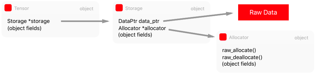
The abstraction responsible for holding the data isn’t actually the Tensor, but the Storage. It holds a pointer to the raw data and contains information such as the size and allocator. Storage is a dump abstraction, there is no metadata telling us how to interpret the data it holds.

struct C10_API StorageImpl : public c10::intrusive_ptr_target {
	...
	DataPtr data_ptr_;
	SymInt size_bytes_;
	Allocator* allocator_;
}

The Storage abstraction is very powerful because it decouples the raw data and how we can interpret it. We can have multiple tensors sharing the same storage, but with different interpretations, also called views, but without duplicating memory.

x = torch.ones((2,2))
x_view = x.view(4)
x_data = x.untyped_storage().data_ptr()
x_view_data = x_view.untyped_storage().data_ptr()
x_data == x_view_data #True

Memory allocators:

The tensor storage can be allocated either in the CPU memory or GPU, therefore a mechanism is required to switch between these different allocations. There are allocators that will use the GPU allocators such as cudaMalloc() when the storage should be used for the GPU or posix_memalign() POSIX functions for data in the CPU memory.

PyTorch uses a CUDA caching allocators that maintains a cache allocations with the Block structure. The torch.cuda.empty_cache() will release all unused blocks.

The Tensor has Storage which in turn has a pointer to the raw data and to the Allocator to allocate memory according to the destination device.

Just-in-time compiler:

PyTorch is eager by design, which means that it is easily hackable to debug, inspect etc. However, this poses problems for optimization and for decoupling it from Python (the model itself is a Python code). PyTorch introduced torch.jit, which has two main methods to convert a PyTorch model to a serializable and optimizable format.

(and others)

Tensors: ndarrays that run on GPUs

The torch.tensor() routine always copies data. If you have a Tensor and want to change its requires_grad flag, use requires_grad_() or detach() to avoid a copy. If you have a numpy array and want to avoid a copy, use torch.as_tensor(). The detach returns a new Tensor, detached from the current graph.

Autograd engine:

torch.autograd is PyTorch’s automatic differentiation engine that powers neural network training. Neural networks (NNs) are a collection of nested functions that are executed on some input data. These functions are defined by parameters (consisting of weights and biases), which in PyTorch are stored in tensors.

Training a NN happens in two steps:

Forward propagation: In forward prop, the NN makes it best guess about the correct output. It runs data through each of its functions to make this guess.

Backward propagation: In backprop, the NN adjusts its parameters proportionate to the error in its guess. It does this by traversing backwards from the output, collecting the derivatives of the error with respect to the parameters of the functions (gradients), and optimizing the parameters using gradient descent.

Example:

We create two tensors a and b with requires_grad=True which signals to autograd that every operation on them should be tracked.

a = torch.tensor([2., 3.], requires_grad=True)
b = torch.tensor([6., 4.], requires_grad=True)

We create another tensor Q from a and b.

Q = 3*a**3 - b**2

When we call .backward() on Q, autograd calculates gradients and stores them in respective tensors’ .grad attribute. We need to explicitly pass a gradient argument in Q.backward() because it is a vector. gradient is a tensor of the same shape as Q, and it represents the gradient of Q w.r.t itself,

Under the hood, each primitive autograd operator is really two functions that operate on Tensors. The forward function computes output Tensors from input Tensors. The backward function receives the gradient of the output Tensors with respect to some scalar value, and computes the gradient of the input Tensors with respect to that same scalar value.

In PyTorch we can easily define our own autograd operator by defining a subclass of torch.autograd.Function and implementing the forward and backward functions. We can then use our new autograd operator by constructing an instance and calling it like a function, passing Tensors containing input data.

external_grad = torch.tensor([1., 1.]) # of Q wrt to a scalar;
Q.backward(gradient=external_grad)

Equivalently, we can also aggregate Q into a scalar and call backward implicitly, like:

Q.sum().backward()

Vector calculus:

Mathematically, if you have a vector function $y = f (x)$ essentially a NN, then gradient of $y$ with respect to $x$ is a Jacobian matrix $J$ :

My Knowledge Base

Explorer