Deep Learning

Probability theory is a mathematical framework for representing uncertain statements. First, the laws of probability tell us how AI systems should reason, so we design our algorithms to compute or approximate various expressions derived using probability theory. Second, we can use probability and statistics to theoretically analyze the behavior of proposed AI systems.

When we say that an outcome has a probability $p$ of occurring, it means that if we repeated the experiment infinitely many times, then a proportion $p$ of the repetitions would result in that outcome. This kind of reasoning does not seem immediately applicable to propositions that are not repeatable. If a doctor analyzes a patient and says that the patient has 40 percent chance of having the flu, this means something very different - we cannot many infinitely many replicas of the patient with the same symptoms. The former kind of probability, related directly to the rates at which events occur, is known as frequentist probability, while the latter, related to qualitative levels of certainty, is known as Bayesian probability.

A random variable is a variable that can take on different values randomly. A probability distribution is a description of how likely a random variable or set of random variables is to take on each of its possible states. The way we describe probability distributions depends on whether the variables are discrete or continuous.

A probability distribution over discrete variables may be described using a probability mass function. Often we associate each random variable with a different probability mass function. The probability mass function maps from a state of a random variable to the probability of that random variable taking on that state.

The probability that $X=x$ is denoted as $P(x)$, with a probability of $1$ indicating that $X=x$ is certain and a probability of $0$ indicating that $X=X$ is impossible. Probability mass function can act on many variables at the same time.

Such a probability distribution over many variables is known as a joint probability distribution $P(X=x,Y=y)$ denotes the probability that $X=x$ and $Y=y$ simultaneously.

Sometimes we know the probability distribution over a set of variable and we want to know the probability distribution over just a subset of them. The probability distribution over the subset is known as the marginal probability distribution. For example, suppose we have discrete random variables $X$ and $Y$, and we know $P(X,Y)$. We can find $P(X)$ with the sum rule: $\forall x\in X,P(X=x)={\sum }_{y}P(X=x,Y=y)$ When the values of $P(X,Y)$ are written in a grid with different values of $x$ in rows and different values of $y$ in columns, it is natural to sum across a row of the grid, then write $P(x)$ in the margin of the paper just to the right of the row.

In many cases, we are interested in the probability of some event, given that some other event has happened. This is called conditional probability. We denote that $Y=y$ given $X=x$ as $P(Y=y|X=x)$. This conditional probability can be computed with the formula: $P(Y=y|X=x)=\frac{P(Y=y,X=x)}{P(X=x)}$ Bayes’ rule:

We often find ourselves in a situation where we know $P(Y|X)$ and need to know $P(X|Y)$. Fortunately, if we also know $P(X)$, we can computed the desired quantity using Bayes’ rule: $P(X|Y)=\frac{P(X)P(Y|X)}{P(Y)}$ Note that while $P(Y)$ appears in the formula, it is usually feasible to compute $P(Y)={\sum }_{x}P(Y|x)P(x)$, so we do not need to begin with knowledge of $P(Y)$,

$P(\text{theory}|\text{evidence})=\frac{P(\text{evidence}|\text{theory})P(\text{theory})}{P(\text{evidence})}$

Expected values:

The expectation of some function $f(x)$ with respect to a probability distribution $P(X)$ is the average, or mean value, that $f$ takes on when $x$ is drawn from $P$. For discrete variables this can be computed with: $E_{x\sim P}[f(x)]={\sum }_{x}P(x)f(x)$ The variance gives a measure of how much the values of function of a random variable $X$ vary as we sample different values of $x$ from its probability distribution: $\text{Var}(f(x))=E[(f(x)-E[f(x)]{)}^2]$ When the variance is low, the values of $f(x)$ cluster near the expected value. The square root of the variance is known as the standard deviation.

The covariance gives sense of how much two values are linearly related to each other, as well as the scale of these variables: $\text{Cov}(f(x),g(y))=E[(f(x)-E[f(x)])(g(y)-E[g(y)])]$ High absolute values of the covariance mean that the values change very much and are both far from their respective means at the same time. If the sign of the covariance is positive, then both variables tend to take on relatively high values simultaneously. If the sign of the covariance is negative, then one variable tends to take on a relatively high value at the times that the other takes on a relatively low value and vice versa. Other measures such as correlation normalize the contribution of each variable in order to measure only how much the variables are related, rather than also being affected by the scale of the separate variables.

The notions of covariance and dependence are related but distinct concepts. They are related because two variables that are independent have zero covariance, and two variables that have nonzero covariance are dependent. Independence, however, is a distinct property from covariance. For two variables to have zero covariance, there must be no linear dependence between them. Independence is a stronger requirement than zero covariance, because independence also excludes nonlinear relationships. It is possible for two variables to be dependent but have zero covariance.

(see also: numpy probabilities)

Information theory:

Information theory of a branch of applied information that revolves around quantifying how much information is present in a signal. The basic intuition behind information theory is that learning that an unlikely event has occurred is more informative than learning that a likely even has occurred. We define the self-information of an event $X=x$ to be: $I(x)=-\lg P(x)$ Our definition of $I(x)$ is written in units of Shannon. One Shannon is the amount of information gained by observing an event of probability $\frac{1}{2}$. Other texts use base-e logarithms and units called nats; information measured in bits is just a rescaling of information measured in nats.

Self-information deals only with a single outcome. We can quantify the amount of uncertainty in an entire probability distribution using the Shannon entropy, $H(x)=E_{x\sim P}[-\lg P(x)]$In other words, the Shannon entropy of a distribution is the expected amount of information in an event drawn from that distribution. It gives a lower bound on the number of bits needed on average to encode symbols drawn from a distribution $P$. Distributions that are nearly deterministic where the outcome is nearly certain have low entropy; distributions that are closer to uniform have high entropy.

events=information expected information in a distribution=entropy

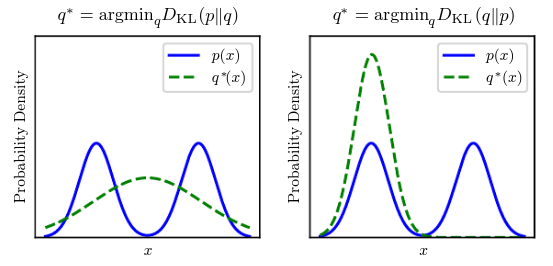
If we have two separate probability distributions $P(X)$ and $Q(X)$ over the same random variable $X$, we can measure how different these two distributions are using the Kullback-Leibler divergence: $D_{KL}(P||Q)=E_{x\sim P}\left[\log P(x)-\log Q(x)\right]$ Relative entropy is only defined in this way if, for all x, $Q(x)=0$ implies $P(x)=0.$ It is often called the information gain achieved if $P$ would be used instead of $Q$ which is currently used. By analogy with information theory, it is called relative entropy of $P$ with respect to $Q$.

def kl_divergence(p, q):
    if np.bitwise_and((q == 0), (p != 0)).any(): return np.inf
    with np.errstate(divide='ignore', invalid='ignore'):
        return np.sum(np.where(p != 0, p * np.log(p / q), 0))

The KL divergence has many useful properties, most notably being non-negative. The KL divergence is $0$ if and only if $P$ and $Q$ are the same distribution in the case of discrete variables. Because the KL divergence is non-negative and measures the difference between two distributions, it is often conceptualized as measuring some sort of distance between these distributions. It is not a true distance because it is not symmetric: $D_{KL}(P||Q)\ne D_{KL}(Q||P)$ for some $P$ and $Q$. This asymmetry means that there are important consequence to the choice of whether to use $P||Q$ or $Q||P$:

A quantity that is related to KL divergence is the cross-entropy $H(P,Q)=H(P)+D_{KL}(P||Q)$, which is similar to the KL divergence but lacking the term on the left: $H(P,Q)=-E_{x\sim P}\log Q(x)$

def cross_entropyp(p, q):
    if np.bitwise_and((q == 0), (p != 0)).any(): return np.inf
    with np.errstate(divide='ignore', invalid='ignore'):
        return np.sum(np.where(p != 0, p*np.log(q), 0))

Minimizing the cross-entropy with respect to $Q$ is equivalent to minimizing the KL divergence, because $Q$ does not participate in the omitted term. When computing many of these quantities, it is common to encounter expressions of form $0\log 0$. By convention, in the context of information theory, we treat these expressions as $0$.

Maximum Likelihood:

Consider a set of $m$ examples $X=\{x^{(1)},\dots ,x^{(m)}\}$ drawn independently from the true but unknown data generating function $p_{\text{data}}(X)$. Let $p_{\text{model}}(X;\theta )$ be a parametric family of probability distributions over the same space indexed by $\theta$. In other words, $p_{\text{model}}(X;\theta )$ maps any configuration $x$ to a real number estimating the true probability $p_{\text{data}}(X)$.

The maximum likelihood estimator for $\theta$ is then defined as: ${\theta }_{ML}={\text{argmax}}_{\theta }{\prod }_{i=1}^m{p}_{\text{model}}(x^{(i)};\theta )$( maximize probabilities of occurrence of observed data )

The product over many probabilities is inconvenient for various reasons. For example, it is prone to numerical overflow. To obtain a more convenient but equivalent optimization problem, we observe that taking the logarithm of the likelihood does not change its arg max but does conveniently transform a product into a sum: ${\theta }_{ML}={\text{argmax}}_{\theta }{\sum }_{i=1}^m\log p_{\text{model}}(x^{(i)};\theta )$ Because the argmax does not change when we re-scale the cost function, we can divide by $m$ to obtain a version of the criterion that is expressed as an expectation with respect to the empirical distribution ${\hat{p}}_{\text{data}}$ defined by the training data: ${\theta }_{ML}={\text{argmax}}_{\theta }{E}_{x\sim p_{\text{data}}}\log p_{\text{model}}(x;\theta )$

One way to interpret maximum likelihood estimation is to view it as minimizing the dissimilarity between the empirical distribution ${\hat{p}}_{\text{data}}$ defined by the training set and the model distribution, with the degree of dissimilarity between the two measured by the KL divergence.

Any loss consisting of a negative log-likelihood is a cross entropy between the empirical distribution defined by the training set and the probability distribution defined by the model. For example, mean squared error is the cross-entropy between the empirical distribution and a Gaussian model. We can thus see maximum likelihood as an attempt to make the model distribution match the empirical distribution ${\hat{p}}_{\text{data}}$. Ideally, we would like to match the true data-generating distribution $p_{\text{data}}$, but we have no direct access to this distribution.

The maximum likelihood estimator can readily be generalized to estimate a conditional probability $P(Y|X;\theta )$ in order to predict $y$ given $x$. This is actually the most common situation because it forms the basis for most supervised learning. If $X$ represents all our inputs and $Y$ all our i.i.d observed targets, then the conditional maximum likelihood estimator can be decomposed into: ${\theta }_{ML}={\text{argmax}}_{\theta }{\sum }_{i=1}^m\log P(y^{(i)}|x^{(i)};\theta )$ In most cases, our parametric model defines a distribution $p(Y|X;\theta )$ and we simply use the principle of maximum likelihood. This means we use the cross-entropy between the training data and the model’s predictions as the cost function. Sometimes, we take a simpler approach, where rather than predicting a complete probability distribution over $Y$, we merely predict some statistic of $Y$ conditioned on $X$. Specialized loss functions enable us to train a predictor of these estimates.

Most modern neural networks are trained using maximum likelihood. This means that the cost function is simply the negative log-likelihood, equivalently described as cross entropy between the training data and the model distribution. This cost function is given by: $J(\theta )=-E_{x,y\sim {\hat{p}}_{\text{data}}}\log p_{\text{model}}(y|x)$The specific form of the cost function changes from model to model, depending on the specific form of $\log p_{\text{model}}$. The expansion of above equation typically yields some terms that do no depend on the model parameters and may be discarded. For example, if $p_{\text{model}}(y|x)=N(y;f(y;f(x;\theta )),I)$, then we recover the mean squared error cost: $J(\theta )=\frac{1}{2}{E}_{x,y\sim {\hat{p}}_{\text{data}}}||y-f(x;\theta )|{|}^2+\text{const}$up to a scaling factor of $1/2$ and a term that does not depend on $\theta$. The discarded constant is based on the variance of the Gaussian distribution, which in this case we chose not to parametrize. An advantage of this approach of deriving cost function from maximum likelihood is that it removes the burden of designing cost functions for each model. Specifying a model $p(y|x)$ automatically determines a cost function $\log p(y|x)$.

The main appeal of the maximum likelihood estimator is that it can be shown to be the best estimator asymptotically, as the number of examples $m\to \infty$, in terms of its rate of convergence as $m$ increases.

One unusual property of the cross-entropy cost used to perform maximum likelihood estimation is that is usually does not have a minimum value when applied to the models commonly used in such a way that they cannot represent a probability of zero or one, but can come arbitrarily close to doing so. For-real valued output variables, if the model can control the density of the output distribution then it becomes possible to assign extremely high density to correct training set output, resulting in cross-entropy approaching negative infinity. Regularization techniques provide several different ways of modifying the learning problem so that the model cannot reap unlimited reward in this way.

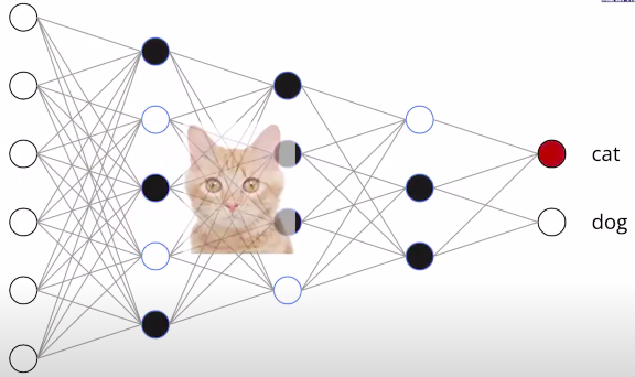
Softmax:

Softmax converts a vector of $K$ real numbers into a probability distribution of $K$ possible outcomes. The standard (unit) softmax function $\sigma :R^K\to (0,1{)}^K$ where $K\ge 1$ is defined by the formula: $\text{sm}(x_i)=\frac{e^{x_i}}{{\sum }_{j=1}^d{e}^{x_j}}$

def softmax(x):
	exp_x = np.exp(x)
	return exp_x/np.sum(exp_x)
 
softmax(np.array([10, 20, 30, 40, 50]))
#[4.24816138e-18 9.35719813e-14 2.06106005e-09 4.53978686e-05 9.99954600e-01]
 
softmax(np.array([1000, 2000, 3000, 4000, 5000]))
#[nan nan nan nan nan]

From the softmax probabilities we can deduce that softmax can become numerically unstable for values with a very large range. Exponentiating a larger number like 10000 leads a very, very large number. This is approximately $2^{10000}$. This causes overflow. A numpy implementation of this stable softmax will look like this:

def softmax(x):
	max_x = np.max(x)
	exp_x = np.exp(x-max_x)
	return exp_x/np.sum(exp_x)
 
softmax(np.array([1000, 2000, 3000, 4000, 5000]))
#[0. 0. 0. 0. 1.]
 
# OR
 
F.softmax(input, dim=None)

Applies to all slices along dim, and will re-sale them so that the elements lie in $[0,1]$.

A critical evaluation of the softmax computation shows a pattern of exponentiation and divisions. We can instead optimize the log softmax. This gives us nice characteristics such as:

• numerical stability
• gradient of log softmax becomes additive
• log is also a monotonically increasing function

The temperature is a way to control entropy of a distribution, while preserving the relative ranks of each event. $\text{sm}(x_i)=\frac{e^{\frac{x_i-c}{\tau }}}{{\sum }_{j=1}^d{e}^{\frac{d_j-c}{\tau }}}$ Cooling it decreases the entropy, accentuating the common events.

Statistical Learning

Statistical learning objects:

Data: A set of $N$ observations $D=\{(x_i,y_i){\}}_{i=1}^N$ drawn i.i.d from an underlying data distribution $P$ over $X\times Y$, where $X$ and $Y$ are respectively the data and label domains.

Approximation Model: The labels $y$ are generated by an unknown function $f^{\ast }$, such that $y_i=f^{\ast }(x_i)$, and the learning problem reduces to estimating the function $f^{\ast }$ using a parameterized function class $F=\{f_{\theta \in \Theta }\}$.

No free lunch: In order to analyse ML algorithms and provide guarantees, we need assumptions on both $X$ and $f^{\ast }$.

Neural networks are a common realization of such parametric classes that typically operate in the so-called interpolating regime, where the estimated $f\in F$ satisfies $f(x_i)=f^{\ast }(x_i)$ for all $i=1,\dots ,N$.

Error metric: Given point-wise convex error measure $L$:

Population Loss: $R(f)=E_{P}L(f(x),f^{\ast }(x))$Empirical Loss:$\hat{R}(f)=\frac{1}{n}{\sum }_{i}L(f(x_i),f^{\ast }(x_i))$For each $f\in F$, $\hat{R}(f)$ is an unbiased estimator of $R(f)$ with variance ${\sigma }^2(f)=\frac{1}{n}{E}_P[L(f(x),f^{\ast }(x))-R(f){]}^2$. However, this point-wise variance bound is not very useful in ML, since hypothesis $f$ depends on training set.

Underlying goal: Minimize $R(f)$ having only access to $\hat{R}(f)$.

Inductive bias via function regularity

Modern machine learning operates with large, high-quality datasets, which, together with appropriate computational resources, motivate the design of rich function classes $F$ with the capacity to interpolate such large data. This mindset plays well with neural networks, since even the simplest choices of architecture yields a dense class of functions. The capacity to approximate almost arbitrary functions is the subject of various Universal Approximation Theorems; several such results were proved and popularised in the 1990s by applied mathematicians and computer scientists.

Universal Approximation, however, does not imply an absence of inductive bias. In order to control fluctuations uniformly, we can define a complexity measure: $c:F\to R_{+}$ and consider the ball $F_{\delta }=\{f\in F;c(f)\le \delta \}$:

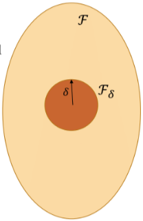
In case neural networks, the complexity measure $c$ can be expressed in terms of network weights. The $L_2$-norm of the network weights, known as weight decay, or the so-called path-norm are popular choices in deep learning literature. More generally, this complexity can be enforced explicitly by incorporating it into the empirical loss (resulting in the so-called Structural Risk Minimisation), or implicitly, as a result of a certain optimisation scheme.

Empirical Risk Minimization: ${\hat{f}}_{\delta }={\text{arg min}}_{f\in F_{\delta }}\hat{R}(f)$ Error decomposition:

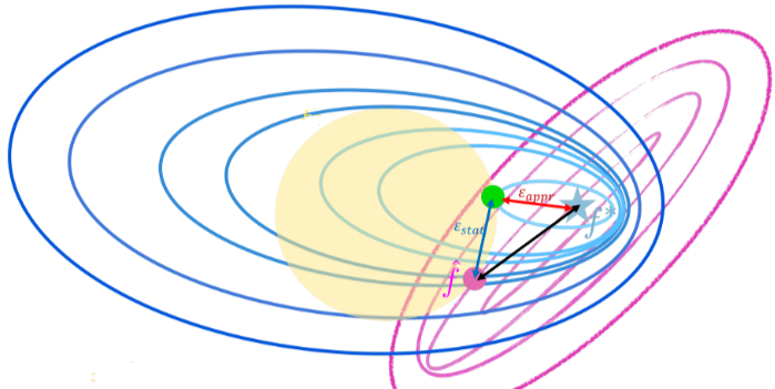
Consider an arbitrary hypothesis $\hat{f}\in F_{\delta }$ for some $\delta >0$. The population error can be decomposed follows: $R(\hat{f})\le {ϵ}_{\text{opt}}+{ϵ}_{\text{stat}}+{ϵ}_{appr}$ Challenges of high dimensional learning: (The volume of hypercube becomes so large that data becomes effectively sparse)

• Approximation error: This is related to how well your hypothesis space can approximate the true underlying function $f^{\ast }$. A smaller hypothesis space (small $\delta$) may not capture the complexity of $f^{\ast }$ well, leading to high approximation error.
• Statistical error: The statistical error is associated with the randomness in the data. It arises because we’re dealing with a finite sample rather than the entire population. The increase in statistical error with $\delta$ is expected because a larger $\delta$ implies a broader set of acceptable functions, making it harder to pinpoint the true underlying function from the training data.

(bias-variance trade-off?)

The use of geometric priors decreases the complexity of the hypothesis class $F_{\delta }$ without discarding useful hypotheses. This should:

• improve statistical error
• not worsen approximation error

Backpropagation:

Depth of a Neural Network

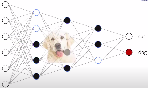
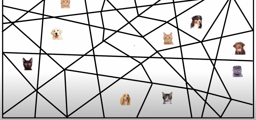
The structure of the network refers to the way its units are arranged. It is specified by the number $n_0$ of input dimensions, the number of layers $L$, and the number of units or width $n_l$ of each layer. We classify the functions computed by different network structures, for different choices of parameters, in terms of their number of linear regions. A linear region of a piecewise linear function $F:R^{n_0}\to R^m$ is a maximal connected subset of the input space $R^{n_0}$, on which $F$ is linear. For the functions that we consider, each linear region has full dimension, $n_0$. There is the common intuition that the number of linear regions of neural networks measures their expressivity.

Rectifier units have two types of behavior; they can be either constant $0$ or linear, depending on their inputs. The boundary between these two behaviors is given by a hyperplane, and the collection of all the hyperplanes coming from all units in a rectifier layers forms a hyperplane arrangement. The hyperplanes in the arrangement split the input into several regions. Each region corresponds to a pattern of OFF/ON ReLUs. More specifically, the activation states are in one-to-one correspondence with the linear regions, i.e., all points in the same linear region activate the same nodes of the DNN, and hence the hidden layers serve as a series of affine transformations of these points.

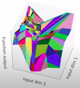
Fixed linear pattern: linear function Different activation patterns: different linear functions

What does depth do?

A map $F$ identifies two neighborhoods $S$ and $S^{\prime }$ of its input domain if it maps them to a common subset $F(S)=F(S^{\prime })$ of its output domain. In this case we also say that $S$ and $S^{\prime }$ are identified by $F$. For example, the four quadrants of 2-D Euclidean space are regions that are identified by the absolute function $g:R^2\to R^2$: $g(x_1,x_2)=[|x_1|,|x_2|{]}^T$. A map $F$ that identifies two subsets $S$ and $S^{\prime }$ can be considered as an operator that folds its domain in such a way that the two subsets $S$ and $S^{\prime }$ coincide and are mapped to the same output. Each hidden layer of a deep neural network can be associated with a folding operator. Each hidden layer folds the space of activations of the previous layer.

In turn, a deep neural network effectively folds its input-space recursively, starting with the first layer. The consequence of this recursive folding is that any function computed on the final folded space will apply to all the collapsed subsets identified by the map corresponding to the succession of foldings. This means that in a deep model any partitioning of the last layer’s image-space is replicated in all input-space regions which are identified by the succession of foldings.

Space foldings are not restricted to foldings along coordinate axes and they do not have to preserve lengths. Instead, the space is folded depending on the orientations and shifts encoded in the input weights W and biases b and on the nonlinear activation function used at each hidden layer. In particular, this means that the sizes and orientations of identified input-space regions may differ from each other.

Upper limit?

The maximal number of linear regions of the functions computed by any rectifier network with a total of $N$ hidden units is bounded from above by $2^N$.

Lower limit?

A rectifier neural network with $n_0$ inputs units and $L$ hidden layers of width $n\ge n_0$ can compute functions that have $\Omega \left({\left(\frac{n}{n_0}\right)}^{(L-1)n_0}{n}^{n_0}\right)$ linear regions.

Thus we can see that the number of linear regions of deep model grows exponentially in $L$ and polynomial in $n$, which is much faster than that of shallow models with $nL$ hidden units.

This framework is applicable to any neural network that has a piecewise linear activation function. For example, if we consider a convolutional neural network with linear rectifier units, we can see that the convolution followed by max pooling at each layer identifier all patches of the input within a pooling region. This will let such a deep convolutional neural network recursively identify patches of the images of lower layers, resulting in exponentially many linear regions of the input space.

But??

Better architectures don’t always require more expressivity:

• Weight sharing reduces expressivity but conveys a useful inductive bias.
• Skip connections keeps expressivity the same.
• Training a shallow network to imitate a deep network (distillation) works well for real tasks.

Width vs depth:

Depth efficiency:

There existence of a 3-layer network, which cannot be realized by any 2-layer to more than a constant accuracy if the size is subexponential in the dimension.

For integer $k$, networks with $O(k^3)$ layers and constant width cannot be realized by any network with $O(k)$ layers whose size is smaller than $2^k$.

Width efficiency:

Currently, neither exponential bound nor the polynomial upper bound seems within the reach for width efficiency.

However, a deep network usually leads to difficulties in optimization, such as the vanishing/exploding gradient problem and shattering gradient problem. (optimization)

activation functions, weight initialization, batch normalization, residual connection;

Another difficulty is that the high complexity caused by the depth can easily result in overfitting. (statistical error)

Depth remedies in PyTorch

These are the basic building blocks for graphs:

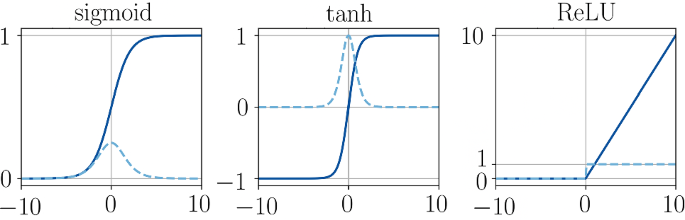
Activation functions:

• Continuously differentiable
• Zero-centered
• Bounded
• Computational cost

Weight initialization:

torch.nn.init.normal_(tensor, mean=0.0, std=1.0)

Xavier, Kiaming etc.

Batch normalization:

Although using Kiaming initializing with any variant of ReLU can significantly reduce the vanishing gradients problems at the beginning of training, it does not guarantee that they won’t come back during training. The Batch Normalization technique consists of adding an operation in the model just before or after the activation function of each hidden layer, simply zero-centering and normalizing each input (so that the scale of the weights can no longer affect the gradients through the layers), then scaling and shifting the result using two new parameter vectors per layer: one for scaling, the other for shifting. In addition, BN also keeps a running count of the Exponential Moving Average (EMA) of the mean and variance. During training, it simply calculates this EMA but does not do anything with it. At the end of training, it simply saves this value as part of the layer’s state, for use during the inference phase.

nn.BatchNorm1d(
	num_features, 
	eps=1e-05, 
	momentum=0.1, 
	affine=True, 
	track_nunning_stats=True
)

• input: $(N,C)$ or $(N,C,L)$, where $N$ is the batch size, $C$ is the number of features, and $L$ is the sequence length.
• output: $(N,C)$ or $(N,C,L)$ (same shape as input).

Applies Batch Normalization over 2D or 3D input: $y=\frac{x-E[x]}{\sqrt{\text{Var}[x]+ϵ}}\ast \gamma +\beta$ The mean and standard-deviation are calculated per-dimension i.e. normalize each feature independently, over the minibatches and $\gamma$ and $\beta$ are learnable parameter vectors of size $C$ (where $C$ is the number of features or channels of the input). By default, the elements $\gamma$ are set to 1 and the elements of $\beta$ are set to 0. At train time in the forward pass, the standard-deviation is calculated via the biased estimator, equivalent to torch.var(input, unbiased=False). However, the value stored in the moving average of the standard-deviation is calculated via the unbiased estimator, equivalent to torch.var(input, unbiased=True). Also by default, during training this layer keeps running estimates of its computed mean and variance, which are then used for normalization during evaluation.

The momentum argument is different from one used in optimize class and the conventional notion of momentum. Mathematically, the update rule for running statistics here is ${\hat{x}}_{\text{new}}=(1-\text{momentum})\ast \hat{x}+\text{momentum}\ast x_t$, where, $\hat{x}$ is the estimated static and $x_t$ is the new observed value..

Dropout:

Dropout allows a DNN to randomly drop some nodes during training and work like an ensemble of several thin networks during inference which mechanism reduces overfitting. If a unit is retained with probability $p$ during training, the outgoing weights of that unit are multiplied by $p$ at inference time. This ensures that for any hidden unit the expected output (under the distribution used to drop units at training time) is the same as the actual output at test time.

nn.Dropout(p=0.5, inplace=False)

• input: $(\ast )$. Input can be of any shape
• Output: $(\ast )$. Output is of the same shape as input

During training, randomly zeros some of the elements of the input tensor with probability p using samples from a Bernoulli distribution. Each channel will be zeroed out independently on every forward call. Furthermore, the outputs are scaled by a factor of $\frac{1}{1-p}$ during training. This means that during evaluation the model simply computes an identity function.

(In terms of linear regions: BN can help DNNs partitions the input space into smaller linear regions, whereas dropout helps around the decision boundaries.)

Skip connections:

The skip connections reparametrise each layer to model a perturbation of the previous feature, rather than a generic non-linear transformation. The resulting residual networks provide several key advantages over previous formulation.

• allow gradient to flow - if weights are close to zero then gradients flow nearly unchanged from layer to layer, which mitigates vanishing/exploding gradient problems
• retain identity information - in a resnet, each layer simply adds information to the original input, so deep layers still have access to structured information about the input (shattered gradients)

The residual paramterisation is consistent with the view that the deep network is a discretisation of an underlying continuous dynamical system, modeled as an ordinary differential equation. Crucially, learning a dynamical system by modeling its velocity turns out to be much easier than learning its position directly. In our learning setup, this translates into an optimization landscape with more favorable geometry, leading to the ability to train much deeper architectures than was possible before. Finally, Neural ODEs are a recent popular architecture that pushes the analogy with ODEs even further, by learning the parameters of the ODE directly and relying on standard numerical integration.

Example:

class ResidualBlock(nn.Module):
	def __init__(self, in_dim, out_dim, dropout_prob=0.0):
		super(ResidualBlock, self).__init__()
		self.linear1 = nn.Linear(in_dim, out_dim)
		self.batch_norm1 = nn.BatchNorm1d(out_dim)
		self.linear2 = nn.Linear(out_dim, out_dim)
		self.batch_norm2 = nn.BatchNorm1d(out_dim)
		self.relu = nn.ReLU()
		self.dropout = nn.Dropout(p=dropout_prob)
	
	def forward(self, x):
		residual = x
		x = self.linear1(x)
		x = self.batch_norm1(x)
		x = self.relu(x)
		x = self.linear2(x)
		x = self.batch_norm2(x)
		x += residual #resnet
		x = self.relu(x)
		x = self.dropout(x) #dropout
		return x
 
class DeepNetwork(nn.Module):
	def __init__(self, 
		hidden_dim=100, no_of_layers=100, 
		use_batch_norm=False, dropout_prob=0.0, use_residual=False):
			super(DeepNetwork, self).__init__()
			self.st = nn.Linear(1, hidden_dim)
			self.ll = nn.ModuleList([ResidualBlock(hidden_dim, hidden_dim) 
				if use_residual else 
				nn.Linear(hidden_dim, hidden_dim, bias=False) 
				for _ in range(no_of_layers)])
			self.use_batch_norm = use_batch_norm
			if self.use_batch_norm:
				self.batch_norms = nn.ModuleList([nn.BatchNorm1d(hidden_dim) 
				for _ in range(no_of_layers)])
			self.ed = nn.Linear(hidden_dim, 1)
			self.relu = nn.ReLU()
			self.dropout = nn.Dropout(p=dropout_prob)
	
	def forward(self, x):
		x = self.relu(self.st(x))
		for i, l in enumerate(self.ll):
			if isinstance(l, ResidualBlock):
				x = l(x)
			else:
				x = l(x)
				if self.use_batch_norm: #pre activations
					x = self.batch_norms[i](x)
				x = self.relu(x)
				x = self.dropout(x) #after activations
		return self.ed(x)

Geometric perspective

The geometric data lives on a domain $\Omega$. The domain is a set, possibly with additional structure. Neural networks for processing geometric data should respect the structure of the data.

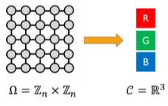
A signal on $\Omega$ is just a function $x:\Omega \to C$, where:

• $\Omega$ is the domain
• $C$ is a vector space whose dimensions are called channels

(numbers to counts: groups to symmetry)

Symmetry groups:

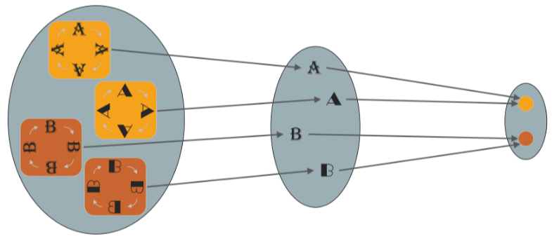
A symmetry of an object is a transformation of that object that leaves it or rather a certain property of said object or system unchanged or invariant. A transformation on a domain $g:\Omega \to \Omega$ is a symmetry if it preserves the structure of $\Omega$.

Any invertible map that respects the class boundaries is a symmetry of the label function $L$. For example: if we knew all the symmetries of the label function $L$, we only need one label per class. If the learning problem is non-trivial, we should not expect to be able to find the full symmetry group a priori.

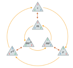
The collection of all symmetries form an algebraic object known as group. Formally, a group is a set $G$ with a binary operation $G\times G\to G$ namely composition satisfying the following properties. Rather than considering groups as abstract entities, we are mostly interested in how groups act on data since we assumed that there is some domain $\Omega$ underlying our data, we will study how the group acts on $\Omega$, and from there obtain actions of the same group on the space of signals $X(\Omega )$.

($g,h$ are group elements $G$, $u$ is a point on $\Omega$)

A group action of $G$ on a set $\Omega$ is a map $G\times \Omega \to \Omega$ denoted $(g,u)\to gu$ associating a group element $g\in G$ and a point $u\in \Omega$ with other point on $\Omega$ in a way that is compatible with the group operations, i.e. $g(hu)=(gh)u$. Given an action of $G$ on $\Omega$, we automatically obtain an action of $G$ on the space of signals $X(\Omega )$: $(gx)(u)=x(g^{-1}u)$ The most important kind of group actions are linear group actions, also known as group representations. The actions on signals is indeed linear. We can describe linear actions by currying as a map, that assigns each $g\in G$ an invertible matrix $\rho (g):G\to R^{n\times n}$, and satisfying the condition $\rho (gh)=\rho (g)\rho (h)$ for all $g,h\in G$. The dimension $n$ of the matrix is in general arbitrary and not necessarily related to the dimensionality of the group or the dimensionality of $\Omega$, but in applications to deep learning $n$ will usually be the dimensionality of the feature space on which the group acts.

Example:

• The group $G=(Z,+)$
• The domain $\Omega =Z_5=\{0,1,2,3,4\}$
• The action of $g=n$ on $u\in \Omega$: $(n,u)\to n+u(\text{mod }5)$
• The representation on $X(\Omega )$:\rho(n)=\left[\begin{array} \\ 0&0&0&0&1 \\ 1&0&0&0&0 \\ 0&1&0&0&0 \\ 0&0&1&0&0 \\ 0&0&0&1&0 \end{array}\right]^n (group: set of g’s compose with $\ast$ and act on $\Omega$ or $X$ with $\rho$. what?)

(symmetry in domain induces symmetry on the functions acting upon it)

(functions must respect the symmetry of domain)

The symmetry of the domain $\Omega$ underlying the signals $X(\Omega )$ imposes structure on the function $f$ defined on such signals. It turns out to be a powerful inductive bias, improving learning efficiency by reducing the space of possible interpolants to those which satisfy the symmetry priors. Symmetries of the domain $\Omega$ captured by group $G$ act on signals $x\in X(\Omega )$ through group representations $\rho (g)$ imposing structure on the functions $f\in F(X(\Omega ))$ acting on such signals.

• A function $f:X(\Omega )\to Y$ is $G-$invariant if $f(\rho (g)x)=f(x)$ for all $g\in G$ and $x\in X(\Omega )$, i.e., its output is unaffected by the group action on the input. Given a hypothesis class $F$, we can make it $G-$invariant by applying the smoothing over group orbits. The linear invariants is not very rich, the family of linear equivariants enables the creation of rich and stable features by composition with appropriate non-linear maps.

• A function $f:X(\Omega )\to X(\Omega )$ is $G-$equivariant if $f(\rho (g)x)=\rho (g)f(x)$ for all $g\in G$ i.e. group action on the input affects the output in the same way. The convolutional layers in CNNs are not shift-invariant but shift-equivariant: in other words, a shift of the input to a convolutional layer produces a shift in the output features maps by the same amount.

The issue of invariance in deep learning:

What symmetries are not group? In many applications, we know a priori that a small deformation of the the signal $x$ should not change the output of $f(x)$ so it is tempting to consider such deformations as symmetries but they do not form a group, and we cannot ask for invariance or equivariance to small deformations only. We can build from this insight by considering a multiscale coarsening of the data domain $\Omega$ into a hierarchy ${\Omega }_1,\dots ,{\Omega }_J$. Since $|\tilde{\Omega }|<<|\Omega |$, coarsening reduces curse of dimensionality fine details are necessary.

The Blueprint:

Let $\Omega$ and ${\Omega }^{\prime }$ be domains, $G$ a symmetry group over $\Omega$, and write ${\Omega }^{\prime }\subseteq \Omega$ if ${\Omega }^{\prime }$ can be considered a compact version of $\Omega$. We define the following building blocks:

1. Linear $G-$equiv layer: $B$: $X(\Omega ,C)\to X({\Omega }^{\prime },C^{\prime })$ satisfying $B(g.x)=g.B(x)$ for all $g\in G$ and $x\in X(\Omega ,C)$

2. Nonlinearity: $\sigma :C\to C^{\prime }$ applied element-wise as $(\sigma (x))(u)=\sigma (x(u))$.

3. Local pooling (coarsening): $P:X(\Omega ,C)\to X({\Omega }^{\prime },C)$ such that ${\Omega }^{\prime }\subseteq \Omega$.

4. $G-$invariant layer (global pooling): $A:X(\Omega ,C)\to Y$ satisfying $A(g.x)=A(x)$ for all $g\in G$ and $x\in X(\Omega ,C)$.

Using these blocks allows constructing $G-$invariant functions $f:X(\Omega ,C)\to Y$ of the form:

$f=A\circ {\sigma }_J\circ B_J\circ P_{J-1}\circ \dots \circ P_1\circ {\sigma }_1\circ B_1$ where the blocks are selected such that the output space of each block matches the input of the space of the next one. Different blocks may exploit different choices of symmetry groups $G$.

Geometric grids

The applications of computer vision, natural language processing, and speech recognition all share a geometric common denominator: an underlying grid structure. The grids are a particular case of graphs with special adjacency. However, since the order of nodes in a grid is fixed, machine learning models for signals defined on grids are no longer required to account for permutation invariance, and have a stronger geometric prior: translation invariance.

The convolution is a translation equivariant linear operation (see?). As discussed in GDL template for general symmetries, extracting translation invariant features out of the convolutional operator $F$ requires a non-linear step. Convolutional features are processed through a non-linear activation function acting element-wise on the inputs. This non-linearity effectively rectifies the signals, pushing their energy towards lower frequencies, and enabling the computation of high-order interactions across scales by iterating the construction.

The CNN and similar architectures had a multiscale structure, where after each convolutional layer one performs a grid coarsening in resolution. This enables multiscale filters with effectively increasing receptive fields, yet retaining a constant number of parameters per scale. Several signal coarsening strategies referred to as pooling may be used, the most common are applying a low-pass anti-aliasing filter e.g. local average followed by grid downsampling, or non-linear max-pooling.

It is also possible to perform translation invariant global pooling operations within CNNs. Intuitively, this involves each pixel - which after, several convolutions, summarizes a patch centered arount it - proposing the final representation of the image, with the ultimate choice of being guided by a form of aggregation of these proposals. A popular choice here is the average function, as its outputs will retain similar magnitudes irrespective of the image size.

Data augmentation:

While CNNs encode the geometric priors associated with translation invariance and scale separation, they do not explicitly account for other known transformations that preserve semantic information, e.g lightning or color changes, or small rotations and dilations. A pragmatic approach to incorporate these priors with minimal architectural changes is to perform data augmentation, where one manually performs said transformations to the input images and adds them into the training set.

Conv2D: Applies a 2D convolution over an input signal composed of several input planes.

nn.Conv2d(in_channels, out_channels, kernel_size, stride=1, padding=0, bias=True)

• input: $(N,C_{\text{in}},H_{\text{in}},W_{\text{in}})$ or $(C_{\text{in}},H_{\text{in}},W_{\text{in}})$

• output: $(N,C_{\text{out}},H_{\text{out}},W_{\text{out}})$ or $(C_{\text{out}},H_{\text{out}},W_{\text{out}})$, where $H_{\text{out}}=\lfloor \frac{H_{\text{in}}+2\times \text{padding}[0]-\text{kernel}[0]}{\text{stride}[0]}\rfloor$ $W_{\text{out}}=\lfloor \frac{W_{\text{in}}+2\times \text{padding}[1]-\text{kernel}[1]}{\text{stride}[1]}\rfloor$

• weight: the learnable weights of the module of shape (out_channels, in_channels, kernel_size[0], kernel_size[1]). The values of these weights are sampled from $U(-\sqrt{k},\sqrt{k})$ where $k=\frac{1}{C_{\text{in}}\ast {\Pi }_{i=0}^1{\text{kernel}}_{\text{size}}[i]}$ .

• bias: the learnable weights of the module of shape (out_channels). If Bias is True, then the values of these wieghts are sampled from $U(-\sqrt{k},\sqrt{k})$ where $k=\frac{1}{C_{\text{in}}\ast {\Pi }_{i=0}^1{\text{kernel}}_{\text{size}}[i]}$ .

MaxPool2D:

nn.MaxPool2d(kernel_size, stride=None, padding=0)
 
nn.AdaptiveMaxPool2d(output_size)

Applies a 2D max pooling over an input signal composed of several input planes.

AvgPool2D:

nn.MaxPool2d(kernel_size, stride=None, padding=0)
 
nn.AdaptiveAvgPool2d(output_size)

Applies a 2D average pooling over an input signal composed of several input planes.

GNNs

A graph is specified with an adjacency matrix $A$ and node features $X$. The permutation equivariant functions $F(X,A)$ are constructed by applying shared permutation invariant functions $\varphi (x_u,X_{N_u})$ over local neighborhoods. Under various guises, this local function $\varphi$ can be referred to as diffusion, propagation, or message passing, and the overall computation of such $F$ as a GNN layer.

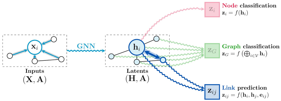
The permutation invariance is ensured by aggregating features from $X_{N_u}$ (potentially transformed by means of some function $\psi$) with some permutation invariant function $\oplus$, and then updating the features of node $u$, by means of some function $\varphi$. Typically, $\varphi$ and $\psi$ are learnable.

The convolutional flavor where the features of the neighborhood nodes are directly aggregated with fixed weights, typically depends on entries in A representing the structure of the graph. $h_u=\varphi \left(x_u,{⨁}_{v\in N_u}{c}_{uv}\psi (x_v)\right)$ Here, $c_{uv}$ are fixed weights, that specify the importance of node $v$ to node $u$‘s representation. Note that when the aggregation operator $\oplus$ is chosen to be the summation, it can be considered as linear diffusion.

The attention flavor where the interactions are implicit: $h_u=\varphi \left(x_u,{⨁}_{v\in N_u}a(x_u,x_v)\psi (x_v)\right)$Here, $a$ is a learnable self-attention mechanism that computes importance coefficients ${\alpha }_{uv}=a(x_u,x_v)$ implicitly. They are often softmax-normalized across all neighbors. When $\oplus$ is the summation, the aggregation is still a linear combination of the neighborhood node features, but now the weights are feature-dependent. Assuming some kind of normalization over the attentional coefficients e.g. softmax, we can constrain all the scalars $a(x_u,x_v)$ to be in the range $[0,1]$; as such, we can think of self-attention as inferring a soft adjacency matrix, $a_{uv}=a(x_u,x_v)$, as a byproduct of gradient-based optimization for some downstream task. Let the GNN choose its own edges!

class SelfAttention(nn.Module):
 
	def __init__(self, embed_size):
		super(SelfAttention, self).__init__()
		self.embed_size = embed_size
		self.q = nn.Linear(embed_size, embed_size, bias=False)
		self.k = nn.Linear(embed_size, embed_size, bias=False)
		self.v = nn.Linear(embed_size, embed_size, bias=False)
 
	def forward(self, x):
		return
		torch.matmul(
				F.softmax(torch.matmul(self.q(x), self.k(x).permute(0, 2, 1)), 
				# features dependent layer weights
				self.v(x)
				# features
			)
		)

MultiheadAttention: Allows the model to jointly attend to information from different representation subspaces.

nn.MultiheadAttention(embed_dim, num_heads, batch_first=False)

• query: Query embeddings of shape $(L,N,E)$ when batch_first=False or $(N,L,E)$ when batch_first=True, where $L$ is the target sequence length, $N$ is the batch size, and $E$ is the query embedding dimension embed_dim.

• key:

• value:

• attn_output: Attention output $(L,N,E)$ when batch_first=False or $(N,L,E)$ when batch_first=True, where $L$ is the target sequence length, $N$ is the batch size, and $E$ is the embedding dimension embed_dim.

• attn_output_weights: Only returned when need_weights=True.

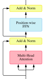
TransformerEncoderLayer: is made up of self-attention and feedforward network.

nn.TransformerEncoderLayer(
						   d_model, 
						   nhead, 
						   dim_feedforward=2048,
						   dropout=0.1,
						   activation=<function relu>,
						   layer_norm_eps=1e-05,
						   batch_first=False,
						   norm_first=False,
					)

• src: the sequence to the encoder layer , $(S,N,E)$ if batch_first=False or $(N,S,E)$ if batch_first=True
• src_mask: the mask for src sequence, $(S,S)$
• is_casual: if specified, applies a casual mask as src_mask. Default: False.

The forward() will use a special optimized implementation Flash Attention if all of the following conditions are met:

• autograd is disabled using torch.inference_mode
• training is disable (using .eval()
• batch_first=True
• activation is one of relu or gelu
• src_mask is passed

(i think nobody uses them anymore)

Recurrent layers

The inputs can also be considered sequential, in which case, we assume that the input consists of arbitrarily many steps, wherein each step $t$ we are provided with an input signal, which we represent as $X^{(t)}\in X({\Omega }^{(t)})$. While in general the domain can evolve in time together with the signals on it, it is typically assumed that the domain is kept fixed across all the $t$. Social networks are an example where one often has to account for the domain changing through time, as new links are regularly created as well as erased. The domain in this setting is often referred to as a dynamic graph.

Often, the individual $X^{(t)}$ inputs will exhibit useful symmetries and hence may be nontrivially treated by any of the architectures. An example include: videos, $\Omega$ is a fixed grid, and signals are a sequence of frames. Let us assume an encoder function $f(X^{(t)})$ providing latent representations at the level of granularity appropriate for the problem and respectful of the symmetries in the input domain. At each timestep, we are given a grid-structured input represented as an $n\times d$ matrix $X^{(t)}$, where $n$ is the number of pixels fixed in time and $d$ is the number of input channels. Further we are interested in analysis at the level of entire frames, in which case it is appropriate to implement $f$ as translation invariant CNN, outputting a $k-$dimensional representation $z^{(t)}=f(X^{(t)})$ of the time frame at time-step $t$.

We are now left with the task of appropriately summarizing a sequence of vectors $z^{(t)}$ across all steps. A canonical way to dynamically aggregate this information in a way that respects the temporal progression of inputs and also easily allows for online arrival of novel data-points is RNN which are an interesting geometric architecture to study in their own right, since they implement a rather unusual type of symmetry over the inputs $z^{(t)}$.

At each step, the recurrent neural network computes an $m-$dimensional summary vector of $h^{(t)}$ of all input steps up to and including $t$. This partial summary is computed conditional on the current step’s features and the previous step’s summary, through a shared update function, $R:R^k\times R^m\to R^m$: $h^{(t)}=R(z^{(t)},h^{(t-1)})$

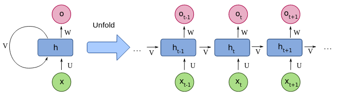
and, as both $z^{(t)}$ and $h^{(t-1)}$ are flat vector representations, $R$ may be most easily expressed as single fully-connected neural networks layer: $h^{(t)}=\sigma (W_{ih}{z}^{(t)}+U_{hh}{h}^{(t-1)}+b)$ where $W\in R^{k\times m}$, $U\in R^{m\times m}$ and $b\in R^m$ are learnable parameters, and $\sigma$ is an activation function. While this introduces loops in the network’s computational graph, in practice the network is unrolled for an appropriate number of steps, allowing for backpropagation through time to be applied.

• input: tensor of shape $(N,L,H_{\text{in}})$
• $h_0$: tensor of shape $(D\ast \text{num of layers},N,H_{\text{out}})$
• output: tensor of shape $(N,L,D\ast H_{\text{out}})$ containing the output features $(h_t)$ from the last layer.
• $h_n$: tensor of shape $(D\ast \text{num of layers},N,H_{\text{out}})$ containing the final hidden state.
• $N$ = batch size, $L$ = sequence length, $D$ = $2$ if bidirectional else $1$, $H_{\text{in}}$= input size, $H_{\text{out}}$ = hidden size.

The time index need not literally refer to the passage of time in the real world, sometimes, it refers only to the position in the sequence. The summary vectors may be appropriately leveraged for the downstream task - if a prediction is required at every step of the sequence, then a shared predictor may be applied at each $h^{(t)}$ individually. For classifying entire sequences, typically the final summary, $h^T$, is passed to a classifier. Here, $T$ is the length of the sequence.

Specially, the initial summary vector is usually either set to the zero-vector, i.e. $h^{(0)}=0$, or it is made learnable. Analyzing the manner in which the initial summary vector is set also allows us to deduce an interesting form of translation equivariance exhibited by RNNs.

The gradient computation involves performing a forward propagation moving left to right through unrolled grpah, followed by a backward propagation pass moving right to left through the graph. The runtime is $O(\tau )$ and cannot be reduced by parallelization.

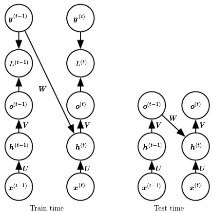
Teacher forcing is a procedure in which during training the model receives the ground truth output $y^{(t)}$ as input at time $t+1$. The maximum likelihood specifies that during training, rather than feeding the model’s own output back into itself, it should be fed with the target values specifying what the correct output should be.

Bidirectional RNNs:

The causal RNN state state at time $t$ captures only information from the past, $z^{(1)},\dots ,z^{(t-1)}$. In many applications, however, a prediction $y^{(t)}$ that may depend on the whole input sequence. Bidirectional combine an RNN that moves forward through time, beginning from the start of the sequence, with another RNN that moves backward through time, beginning from the end of the sequence.

A typical bidirectional RNN with $h^{(t)}$ standing for the state of the sub-RNN that moves forward through time and $g^{(t)}$ standing for the state of the sub-RNN that moves backward through time:

Any symmetry?

Since we interpret the individual steps $t$ as discrete time-steps, the input vectors $z^{(t)}$ can be seen living on a one-dimensional grid of time-steps. While it might be attractive to attempt extending our translation equivariance analysis from CNNs here, it cannot be done in a trivial manner.

To see why, let us assume that we have produced a new sequence $z^{\prime (t)}=z^{(t+1)}$ by performing a left shift of our sequence by one step. It might be tempting to attempting to show $h^{\prime (t)}=h^{(t+1)}$, as one expects with translation equivariance; however, this will not generally hold. Consider $t=1$; directly applying and expanding the update function, we recover the following: h'^{(1)}=R(z'^{(1)}, h^{(0)})=R(z^{(2)}, h^{(0)})$$$$h^{(2)}=R(z^{(2)},h^{(1)})=R(z^{(2)}, R(z^{(1)},h^{(0)}))Hence, unless we can guarantee that $h^{(0)}=R(z^{(1)},h^{(0)})$ we will not recover translation equivariance. Similar analysis can be done for steps $t>1$. Fortunately, with a slight refactoring of how we represent $z$, and for a suitable choice of $R$, it is possible to satisfy the equality above, and hence demonstrate a setting in which RNNs are equivariant to shifts. Our problem was largely one of boundary conditions: the equality above includes $z^{(1)}$, which our left shifted operation destroyed. To abstract this problem away, we will observe how an RNN processes an appropriately left-padded sequence ${\bar{z}}^{(t)}$, defined as follows: \bar{z}^{(t)}=\left\{\begin{array}\\0&t\le t'\\z^{(t-t')}&t>t'\end{array}\right. Such a sequence now allows for left-shifting by up to $t^{\prime }$ steps without destroying any of the original input elements. Further, note we do not need to handle right-shifting separately; indeed, equivariance to right shifts naturally follows from RNN equations.

We can now again analyse the operation of the RNN over a left-shifted version of ${\bar{z}}^{(t)}$, which we denote by ${\bar{z}}^{\prime }(t)={\bar{z}}^{(t+1)}$ as we did earlier: $h^{\prime (1)}=R({\bar{z}}^{\prime (1)},h^{(0)})=R({\bar{z}}^{(2)},h^{(0)})$ $h^{(2)}=R(z^{(2)},h^{(1)})=R(z^{(2)},R(0,h^{(0)}))$ where the substitution ${\bar{z}}^{(1)}=0$ holds as long as $t^{\prime }\ge 1$, i.e. as long as any padding is applied. Now, we can guarantee equivariance to left-shifting by one step $h^{\prime (t)}=h^{(t+1)}$ as long as $h^{(0)}=R(0,h^{(0)})$. Said differently, $h^{(0)}$ must be chosen to be a fixed point of a function $\gamma (h)=R(0,h)$. If the update function $R$ is conveniently chosen, then not only can we guarantee existence of such fixed points, but we can directly obtain them by iterating the application of $R$ until convergence; e.g. as follows: $h_0=0,h_{k+1}=\gamma (h_k)$ where the index $k$ refers to the iteration of $R$ in our computation. If we choose $R$ such that $\gamma$ is a contraction mapping, such an iteration will indeed converge to a unique fixed point. Contractions are functions $\gamma :X\to X$ such that, under some norm $||.||$ on $X$, applying $\gamma$ contracts the distance between points: for all $x,y\in X$, and some $q\in [0,1)$, it holds that $||\gamma (x)-\gamma (y)||\le q||x-y||$. Iterating such a function then necessarily converges to a unique fixed point.

Depth in RNNs: It is easy to stack multiple RNNs simply use the $h^{(t)}$ vectors as an input sequence for a second RNN. The occasionally called a deep RNN is potentially misleading effectively due to the repeated application of the recurrent operation, even a single layer RNN layer has depth equal to the number of input steps. This often introduces challenging learning dynamics when optimizing RNNs. The most prominent of such issues is that of vanishing and exploding gradients.

Gated layers

The mathematical challenge of learning long-term dependencies in recurrent network is that gradients propagated over many stages tend to either vanish or explode with much damage to the optimization. A key invention that significantly reduced the effects of vanishing gradients in RNNs is that of gating mechanisms, which allow the network to selectively overwrite information in a data-driven way. Prominent examples of these gated RNNs include the LSTM and the GRU.

The gated RNNs are based on the idea of creating paths through time that have derivatives that neither vanish nor explode.

The LSTM augments the recurrent computation by introducing a memory cell, which stores cell state vectors, $c^{(t)}\in R^m$, that are preserved between computational steps. The LSTM computes summary vectors, $h^{(t)}$, directly based on $c^{(t)}$, and $c^{(t)}$ is, in turn, computed using $z^{(t)}$, $h^{(t-1)}$ and $c^{(t-1)}$. Critically the cell is not completely overwritten based on $z^{(t)}$ and $h^{(t-1)}$, which would expose the network to the same issues as the simple RNN. Instead a certain quantity of the previous cell state may be retained - and the proportion by which this occurs is explicitly learned from data.

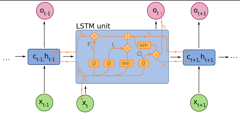
A common LSTM unit is composed of a cell, an input gate, an output gate and a forget gate:

• a context cell $c_t$ remembers values over arbitrary time intervals

• forget gate decides what information to discard from a previous state by assigning a previous state, compared to a current input, a value between $0$ and $1$, where a rounded value of $1$ means to keep the information and a value of $0$ means to discard it

• input gate decides which pieces of new information to store in the current state, using the same system as forget gates

• output gate control which pieces of information in the current state to output by assigning a value $0$ to $1$ to the information, considering previous and current states.

Just like in SimpleRNN, we compute features by using a single fully-connected neural network layer over the current input step and previous summary: ${\tilde{c}}^{(t)}=\tanh (W_{ic}{z}^{(t)}+U_{ic}{h}^{(t-1)}+b_c)$But, as mentioned, we do not allow all of this vector to enter the cell - hence why we call it the vector of candidate features, and denote is as ${\tilde{c}}^{(t)}$. Instead, the LSTM directly learns gating vectors, which are real-valued vectors in the range $[0,1]$ and decide how much of the signal should be allowed to enter, exit, and overwrite the memory cell.

Three such gates are computed, all based on $z^{(t)}$ and $h^{(t-1)}$:

• the input gate $i^{(t)}$, which computes the proportion of the candidate vector allowed to enter the cell;
• the forget gate $f^{(t)}$, which computes the proportion of the previous cell state to be retained, and
• the output gate $o^{(t)}$, which computes the proportion of the new cell state to be used for the final summary vector: $i^{(t)}=\text{Logistic}(W_i{z}^{(t)}+U_i{h}^{(t-1)}+b_i)$ $f^{(t)}=\text{Logistic}(W_f{z}^{(t)}+U_f{h}^{(t-1)}+b_f)$ $o^{(t)}=\text{Logistic}(W_o{z}^{(t)}+U_o{h}^{(t-1)}+b_o)$ Finally, these gates are appropriately applied to decode the new cell state, $c^{(t)}$, which is then modulated by the output gate to produce the summary vector $h^{(t)}$, as follows: $c^{(t)}=i^{(t)}\circ {\tilde{c}}^{(t)}+f^{(t)}\circ c^{(t-1)}$ $h^{(t)}=o^{(t)}\circ \tanh (c^{(t)})$ The GRU differ with LSTM in that a single gating unit simultaneously controls the forgetting factor and the decision to update the state unit.

Besides tackling the vanishing gradient issues head-on, it turns out that gated RNNs also unlock a very useful form of invariance to time-warping transformations, which remains out of reach to SimpleRNNs.

Time warping:

We start by illustrating, in a continuous time setting, what does it mean to warp time, and what is required of a recurrent model in order to achieve invariance to such transformations. Let us assume a continuous time-domain signal $z(t)$, on which we would like to apply an RNN. To align the RNN’s discrete-time computation of summary vectors $h^{(t)}$ with an analogue in the continuous domain, $h(t)$, we will observe its linear Taylor expansion: $h(t+\delta )\sim h(t)+\delta \frac{dh(t)}{dt}$ and, setting $\delta =1$, we recover a relationship between $h(t)$ and $h(t+1)$, which is exactly what the RNN update function $R$ computes. Namely, the RNN update function satisfies the following differential equation: $\frac{dh(t)}{dt}=h(t+1)-h(t)=R(z(t+1),h(t))-h(t)$ We would like the RNN to be resilient to the way in which the signal is sampled (e.g. by changing the time unit of measurement), in order to account for any imperfections or irregularities therein. Formally we denote a time warping operation $\tau :R^{+}\to R^{+}$, as any monotonically increasing differentiable mapping between times. Such warping operations can be simple, such as time rescaling; e.g. $\tau (t)=0.7t$ which, in discrete setting, would amount to new inputs being received $\sim 1.43$ steps.

Further, we state that a class of models is invariant to time warping if, for any model of the class and any such $\tau$, there exists another possibly the same model from the class that processes the warped data in the same way as the original model did in the non-warped case. This is a potentially very useful property. If we have an RNN class capable of modelling short-term dependencies well, and we can also show that this class is invariant to time warping, then we know it is possible to train such a model in a way that will usefully capture long-term dependencies as well (as they would correspond to a time dilation warping of a signal with short-term dependencies). As we will shortly see, it is no coincidence that gated RNN models such as the LSTM were proposed to model long-range dependencies. Achieving time warping invariance is tightly coupled with presence of gating mechanisms, such as the input/forget/output gates of LSTMs.

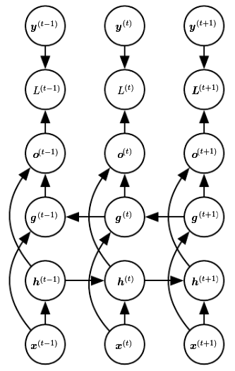
When time gets warped by $\tau$, the signal observed by the RNN at time $t$ is $z(\tau (t))$ and, to remain invariant to such warpings, it should predict an equivalently-warped summary function $h(\tau (t))$. Using Taylor arguments once more, that the RNN update $R$ should satisfy: $\frac{dh(\tau (t))}{d\tau (t)}=R(z(\tau (t+1)),h(\tau (t)))-h(\tau (t))$ However, the above derivative is computed with respect to the warped time τ (t), and hence does not take into account the original signal. To make our model take into account the warping transformation explicitly, we need to differentiate the warped summary function with respect to $t$. Applying the chain rule, this yields the following differential equation: $\frac{dh(\tau (t))}{dt}=\frac{dh(\tau (t))}{d\tau (t)}\frac{d\tau (t)}{dt}=\frac{d\tau (t)}{dt}R(z(\tau (t+1)),h(\tau (t)))-\frac{d\tau (t)}{dt}h(\tau (t))$ and for our continuous-time RNN to remain invariant to any time warping $\tau (t)$, it needs to be able to explicitly represent the derivative $\frac{d\tau (t)}{dt}$, which is not assumed known upfront. We need to introduce a learnable function $\Gamma$ which approximates this derivative. For example, $\Gamma$ could be a neural network talking into account $z(t+1)$ and $h(t)$ and predicting scalar outputs.

Now, remark that, from the point of view of a discrete RNN model under time warping, its input $z^{(t)}$ will correspond to $z(\tau (t))$ and its summary $h^{(t)}$ will correspond to $h(\tau (t))$. To obtain the required relationship of $h^{(t)}$ to $h^{(t+1)}$ in order to remain invariant to time warping, we will use a one-step Taylor expansion of $h(\tau (t))$: $h(\tau (t+\delta ))\sim h(\tau (t))+\delta \frac{dh(\tau (t))}{dt}$ and, once gain, setting $\delta =1$ and substituting the above form then discretising: $h^{(t+1)}=h^{(t)}+\frac{d\tau (t)}{dt}R(z^{t+1},h^{(t)})-\frac{d\tau (t)}{dt}{h}^{(t)}$ $h^{(t+1)}=\frac{d\tau (t)}{dt}R(z^{t+1},h^{(t)})+\left(1-\frac{d\tau (t)}{dt}\right)h^{(t)}$ Finally, we swap $\frac{d\tau (t)}{dt}$ with the aforementioned learnable function $\Gamma$. This gives us the required form for our time warping-invariant RNN: $h^{(t+1)}=\Gamma (z^{(t+1)},h^{(t)})R(z^{(t+1)},h^{(t)})+(1-\Gamma (z^{(t+1)},h^{(t)}))h^{(t)}$ The simple RNNs are not time warping invariant, given that they do not feature the second term, instead they fully overwrite $h^{(t)}$ with $R(z^t,h^{(t)})$, which corresponds to assuming no time warping at all.

Further, our link between continuous-time RNNs and the discrete RNN based on $R$ rested on the accuracy of the Taylor approximation, which holds only if the time-warping derivative is not too large. The intuitive explanation of this is: if our time warping operation ever contracts time in a way that makes time increments $(t\to t+1)$ large enough that intermediate data changes are not sampled, the model can never hope to process time-warped inputs in the same way as original ones—it simply would not have access to the same information. Conversely, time dilations of any form (which, in discrete terms, correspond to interspersing the input time-series with zeroes) are perfectly allowed within our framework.

Combined with our requirement of monotonically increasing $\tau$, we can bound the output space of $\Gamma$ as $0<\Gamma (z^{t+1},h^t)<1$, which motivates the use of logistic sigmoid activation for $\Gamma$: $\Gamma (z^{t+1},h^t)=\text{Logistic}(W_{\Gamma }{z}^{(t+1)}+U_{\Gamma }{h}^{(t)}+b_{\Gamma }$ exactly matching the LSTM gating equations. The main difference is that LSTMs compute gating vectors, whereas ^ equation implies $\Gamma$ should output a scalar. Vectorized gates allow to fit a different warping derivative in every dimension of $h^{(t)}$ allowing for reasoning over multiple time horizons simultaneously. By requiring our RNN class is invariant to non-destructive time warping, we have derived the necessary form that it must have, and showed that it exactly corresponds to the class of gated RNNs. The gates’ primary role under this perspective is to accurately fit the derivative $\frac{d\tau (t)}{dt}$ of the warping transformation.

The notion of class invariance is somewhat distinct from the invariances we studied previously. Namely, once we train a gated RNN on a time warped input with ${\tau }_1(t)$, we typically cannot zero-shot transfer it to a signal warped by a different ${\tau }_2(t)$. Rather, class invariance only guarantees that gated RNNs are powerful enough to fit both of these signals in the same manner, but potentially with vastly different model parameters.