Data Mining

Data mining is the process of extracting and discovering useful information and patterns in large data repositories. We live in a world where vast amounts of data are collected daily. Analyzing such data is an important need.

Not all information discovery tasks are considered to be data mining. For example, looking up individual records using a database management system or finding particular Web pages via a query to an Internet search engine are tasks related to the area of information retrieval.

Data rich information poor situation.

*Challenges?

• Scalability
• High dimensionality
• Heterogeneous and complex data:
• Data ownership and distribution
• Non-traditional analysis:

Steps?

1. Data cleaning: to remove noise and inconsistent data
2. Data integration: where multiple data sources may be combined
3. Data selection: where data relevant to the analysis task are retrieved from the database
4. Data transformation: where data are transformed and consolidated into forms appropriate for mining by performing summary of aggregation operations
5. Data mining: an essential process where intelligent methods are applied to extract data patterns
6. Pattern evaluation: to identify truly interesting patters representing knowledge based on interestingness measures
7. Knowledge representation: where visualization and knowledge representation techniques are used to present mined knowledge to user

Steps 1 through 4 are different forms of data preprocessing, where data are prepared for mining. The data mining step may interact with the user or a knowledge base. The interesting patterns are presented to the user and may be stored as new knowledge in the knowledge base.

Datasets

Data sets are made up of data objects. A data object represents an entity - in a sales database, the objects may be customers, the objects may be customers, store items, and sales; in a medical database, the objects may be patients; in a university database, the objects may be students, professors, and courses.

Data objects are typically described by attributes. If the data objects are stored in a database, they are data tuples. That is, the rows of a database correspond to the data objects, and the columns correspond to the attributes.

An attribute is a data field, representing a characteristic or feature of a data object. Observed values for a given attribute are known as observations. A set of attributes used to describe a given object is called an attribute vector (or feature vector).

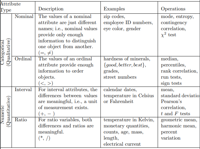
• Nominal attributes: The value of nominal attribute are symbols or name of things. Each value represents some kind of category, code, or state, and so nominal attributes are also referred to as categorical.

• Binary attributes, is a nominal attribute with only two categories or states: 0 or 1, where 0 typically means that the attribute is absent, and 1 means that it is present.

• Ordinal attributes: An ordinal attribute is an attribute with possible values that have a meaningful order or ranking among them, but the magnitude between successive values is not known.

• Numeric attributes: A numeric attribute is quantitative; that is, it is a measurable quantity, represented in integer or real values.

Data visualization

Data visualization aims to communicate data clearly and effectively through graphical representation. More popularly, we can take advantage of visualization techniques to discover data relationships that are otherwise not easily observable by looking at the raw data.

Graphical Plots

…

Similarity and Dissimilarity

In data mining applications, we need ways to assess how alike or unalike objects are in comparison to one another.

Suppose that we have $n$ objects described by $p$ attributes also called measurements. The objects may be tuples in a relational database, and are also referred to as feature vectors. The Dissimilarity matrix stores a collection of proximities that are available for all pairs of $n$ objects. It is often represented by an n-by-n table:

d(n,1) & d(n, 2) & \ldots & \ldots & 0 \end{array}\right]$$ where $d(i,j)$ is the measured dissimilarity between objects $i$ and $j$. In general $d(i, j)$ is a non-negative number that is close to $0$ when objects $i$ and $j$ are highly similar or near each other, and becomes larger the more they differ. 1. Nominal Attributes: The dissimilarity between two objects $i$ and $j$ can be computed based on the ratio of mismatches: $$ d(i,j) = \frac{p-m}{p} $$where, $m$ is the number of matches, i.e. the number of attributes for which $i$ and $j$ are in the same state, and $p$ is the total number of attributes describing the objects. 2. Symmetric Binary Attributes: For symmetric binary attributes, each state is equally valuable. If objects $i$ and $j$ are described by symmetric binary attributes, then the dissimilarity between $i$ and $j$ are: $$d(i,j)= \frac{r+s}{q+r+s+t}$$where, $q$ is the number of attributes that equal $1$ for both objects $i$ and $j$, $r$ is the number of attributes that equal $0$ for object $i$ but equal $1$ for object j, $s$ is the number of attributes that that equal $0$ for object $i$ but $1$ for object $j$, and $t$ is the number of attributes that equal $0$ for both objects $i$ and $j$. 3. Asymmetric Binary Attributes: For asymmetric binary attributes, the two states are not equally important. Given two asymmetric binary attributes, the agreement of two $1$s (a positive match) is then considered more significant than that of two $0$s (a negative match). $$d(i,j)= \frac{r+s}{q+r+s}$$ The coefficient $s(i,j)$ is called the Jaccard coefficient. 4. Numerical Attributes: Let $i=(x_{i1}, x_{i2}, \ldots, x_{ip})$ and $j=(x_{j1}, x_{j2}, \ldots, x_{jp})$ be two objects described by $p$ numeric attributes. - Malinowski, $$d(x,y) = \left(\sum_{k=1}^n |x_k-y_k|^r\right)^\frac{1}{r}$$ - Manhattan $r = 1$, $$d(x,y) = |x_1-y_1| + \ldots + |x_k-y_k| $$ - Supreme $r = \infty$, $$d(x,y) = \text{max}_f |x_f-y_f|$$ - Euclidean $r = 2$, $$d(x,y) = \sqrt{|x_1-y_1|^2 + \ldots + |x_k-y_k|^2}$$ Both the Euclidean and the Manhattan distance satisfy the following mathematical properties: - Positivity: $d(i,i) \ge 0$ - Identify: $d(i,i)=0$ - Symmetry: $d(i,j) = d(j,i)$ - Triangle Inequality: $d(i,j) \le d(i,k) + d(k,j)$ - Cosine Jaccardian Similarity, $$s(i,j) = \frac{i\cdot j}{||i||~||j||}$$ ## Data Preprocessing Real-world databases are highly susceptible to noisy, missing, and inconsistent data due to their typically huge size often several gigabytes or more and their likely origin from multiple, heterogeneous sources. Low-quality data will lead to low-quality mining results. Data have quality if they satisfy the requirements of the intended use. There are many factors comprising data quality, including: - Accuracy: - incorrect attribute values - faulty instruments - human or computer data entry errors - purposefully submit incorrect data values - defaulted values - data transmission errors - technological limits - naming conventions or data codes - Completeness: - not considered important at the time - misunderstanding - equipment malfunctions - deleted due to inconsistencies - Consistency: - Timeliness: - Believability: - Interpretability: ### Data Cleaning Real-world data tend to be incomplete, noisy, and inconsistent. Data cleaning (or data cleansing) routines attempt to fill in missing values, smooth out noise while identifying outliers, and correct inconsistencies in the data. 1. Noisy data: - Regression - Smoothing by means - Anomaly detection techniques 2. Missing values: - Ignore the tuple - Fill in the missing value manually - Use a global constant to fill in the missing value - Use a measure of central tendency for the attribute - Use the most probable value to fill in the missing value Methods 3 to 5 bias the data - the filled-in value may not be correct. Method 5, however, is a popular strategy. In comparison to the other methods, it uses the most information from the present data to predict missing values. ### Data Transformation and Discretization The data are transformed or consolidated so that the resulting mining process may be more efficient, and the patterns found may be easier to understand. 1. Normalization: The measurement unit used can affect the data analysis. In general, expressing an attribute in smaller units will lead to a larger range for that attribute, and thus tend to give such an attribute greater effect. To help avoid dependence on the choice of measurement units, the data should be normalized which involves transforming the data to fall within a smaller or common range such as $[−1,1]$ or $[0.0, 1.0]$. Normalizing the data attempts to give all attributes an equal weight. - Z-score - Min-max - Decimal scaling 2. Discretization: - Width and frequency binning: 3. Binarization: 4. Attribute construction: ### Data Reduction Complex data analysis and mining on huge amounts of data can take a long time, making such analysis impractical or infeasible. 1. Dimensionality reduction is the process of reducing the number of random variables or attributes under consideration. - Attribute subset selection - Wavelet Transforms - [[PCA and SVD]] 2. Numerosity reduction techniques replace the original data volume by alternative, smaller forms of data representation. - Sampling - Data cube aggregation: 3. Data compression are applied so as to obtain a reduced or compressed representation of the original data. If the original data can be reconstructed from the compressed data without any information loss, the data reduction is called lossless. #### Sampling 1. Sampling can be used as a data reduction technique because it allows a large data set to be represented by a much smaller random data sample. Suppose that a large data set, D, contains N tuples. - Sample random sample without replacement: - Sample random sample with replacement: - Stratified sample: If D is divided into mutually disjoint parts called strata, a stratified sample of D is generated by obtaining an SRS at each stratum. This helps ensure a representative sample, especially when the data are skewed. For example, a stratified sample may be obtained from customer data, where a stratum is created for each customer age group. In this way, the age group having the smallest number of customers will be sure to be represented. 2. Attribute subset selection reduces the data set size by removing irrelevant or redundant attributes. The goal of attribute subset selection is to find a minimum set of attributes such that the resulting probability distribution of the data classes is as close as possible to the original distribution obtained using all attributes. ### Data Integration Data mining often requires data integration—the merging of data from multiple data stores. Careful integration can help reduce and avoid redundancies and inconsistencies in the resulting data set. 1. Redundancy analysis - $\chi^2$ test for nominal attributes - Correlation coefficient 2. Tuple duplication 3. Data value conflict detection and resolution ## Data Cube The multidimensional data model views data in the form of a data cube. The starting point is usually a tabular representation of the data, which is called a fact table. Facts are numeric measures. Think of them as the quantities by which we want to analyze relationships between dimensions. Each dimension may have a table associated with it, called dimension table, which further describes the dimension. Two steps are necessary in order to represent data as a multidimensional array: - identification of the dimensions - identification of an attribute that is the focus of the analysis. ![[Pasted image 20230926220532.png]] The dimensions are categorical attributes or continuous attributes that have been converted to categorical attributes. The values of an attribute serve as indices into the array for the dimension corresponding to the attribute. In the Iris example, each attribute had three possible values, and thus, each dimension was of size three and could be indexed by three values. The contents of each cell represents the value of a target quantity (target variable or attribute) that we are interested in analyzing. In the Iris example, the target quantity is the number of flowers whose petal width and length fall within certain limits. The target attribute is quantitative because a key goal of multidimensional data analysis is to look aggregate quantities, such as totals or averages. 1. First, identify the categorical attributes to be used as the dimensions and a quantitative attribute to be used as the target of the analysis. 2. Each row (object) in the table is mapped to a cell of the multidimensional array. The indices of the cell are specified by the values of the attributes that were selected as dimensions, while the value of the cell is the value of the target attribute. 4. Cells not defined by the data are assumed to have a value of 0. A key motivation for taking a multidimensional viewpoint of data is the importance of aggregating data in various ways. In the sales example, we might wish to find the total sales revenue for a specific year and a specific product. Or we might wish to see the yearly sales revenue for each location across all products. Computing aggregate totals involves fixing specific values for some of the attributes that are being used as dimensions and then summing over all possible values for the attributes that make up the remaining dimensions. Given a set of dimensions, we can generate a cuboid (aggregate?) for each of the possible subsets of the given dimensions. The result would form a lattice of cuboids, each showing the data at a different level of summarization. The lattice of cuboids is the data cube. A multidimensional representation of the data, together with all possible aggregates is known as a data cube. ![[Pasted image 20230926222308.png]] A key point is that there are a number of different totals (aggregates) that can be computed for a multidimensional array, depending on how many attributes we sum over. Assume that there are $n$ dimensions and that the $i$th dimension has $s_i$ possible values. If we sum over dimension $j$, then we obtain $s_1\times \ldots \times s_{j-1}\times s_{j+1}\times \ldots \times s_n$ totals, one for each possible combination of attribute values of the $n-1$ other attributes. The totals that result from summing over one attribute form a multidimensional array of $n−1$ dimensions and there are $n$ such arrays of totals. Operations: 1. Pivoting: is a visualization operation that rotates the data axes to view to provide an alternative data representation 2. Slicing and dicing: Slicing is selecting a group of cells from the entire multidimensional array by specifying value for one or more dimension. Dicing involves selecting a subset of cells by specifying a range of attribute values. This is equivalent to defining a subarray from the complete array. In practice, both operations can also be accompanied by aggregation over some dimensions. 3. Roll-up and drill-down: Often categories can be organized as a tree or lattice also known as concept hierarchy. For instance, years consist of months or weeks, both of which consist of days. Locations can be divided into nations, which contain states (or other units of local government), which in turn contain cities. This hierarchical structure gives rise to the roll-up and drill-down operations. To illustrate, starting with the original sales data, which is a multidimensional array with entries for each date, we can aggregate (roll up) the sales across all the dates in a month. Conversely, given a representation of the data where the time dimension is broken into months, we might want to split the monthly sales totals (drill down) into daily sales totals. Of course, this requires that the underlying sales data be available at a daily granularity. ![[Pasted image 20230926225427.png]] The most common modelling paradigm is the star schema, in which the data warehouse contains - a fact table containing the bulk of the data with no redundancy, - a set of smaller dimension tables, one for each dimension. ![[Pasted image 20230926223658.png]] A star schema where sales are considered along four dimensions: time, item, branch, and location. The schema contains a central fact table for sales that contains keys to each of the four dimensions, along with two measures: dollars_sold and units_sold. To minimize the size of the fact table, dimension identifiers (e.g., time key and item key) are system-generated identifiers. ## PCA ... ## Classification Classification is the task of learning a target function $f:x\rightarrow y$ maps each attribute set $x$ to one of predefined discrete class labels $y$. The target function is also known informally as a classification model. The input data for a classification task is a collection of records. Each record, also known as an instance or example, is characterized by a tuple $(x,y)$, where $x$ is the attribute set and $y$ is a designated class label. Each technique employs a learning algorithm to identify a model that best fits the relationship between the attribute set and class label of the input data. ![[Pasted image 20230926233506.png]] Evaluation of the performance of a classification model is based on the counts of test records correctly and incorrectly predicted by the model. These counts are tabulated in a table known as confusion matrix. ![[confusion_matrix.png]] is a useful tool for analyzing how well the classifier can recognizes tuples of different classes, TP and TN tell us when the classifier is getting things right, while FP and FN tell us when the classifier is getting things wrong. The accuracy of a classifier on a given test is the percentage of test tuples that are correctly classified by the classifier. The class Imbalance problem where the main class of interest is rare, i.e. the data set distribution reflects a significant majority of negative class and a minority of positive class. In medical data, there may be a rare class, such as cancer. Suppose that you have trained a classifier to classify medical data tuples, where the class label attribute is cancer and the possible class values are yes and no. An accuracy rate of, say, 97% may make the classifier seem quite accurate, but what if only, say, 3% of the training tuples are actually cancer? Need measures to access how well the classifier can recognize the positive tuples (cancer = yes) and how well it can recognize the negative tuples (cancer = no). Sensitivity and specificity are used to access how well the classifier can recognize the positive tuples (cancer = yes) and how well it can recognize the negative tuples (cancer = no). The precision and recall are also widely used in classification, precision can be thought of as a measure of exactness i.e. what percentage of tuples labeled as positive are actually such, whereas recall is a measure of completeness what percentage of positive tuples are labeled as such. $$\text{precision }= \frac{TP}{TP+FP},~\text{recall (TPR)}= \frac{TP}{TP+FN}$$ In addition to accuracy-based measures, classifiers can also be compared with repsect to following aspects: - Speed - Robustness - Scalability - Interpretability ## Decision Trees We can solve a classification problem by asking a series of carefully crafted questions about the attributes of the test record. Each time we receive an answer, a follow-up question is asked until we reach a conclusion about the class label of the record. The series of questions and their possible answers can be organized in the form of a decision tree, which is a hierarchical structure consisting of nodes and directed edges. - A root node is the starting point. - Leaf or terminal nodes are assigned a class label. - Internal nodes contain attribute test conditions to separate records that have different characteristics. ![[Pasted image 20230927013416.png]] *How to build a decision tree?* In principle, there are exponentially many decision trees that can be constructed from a given set of attributes. While some of the trees are more accurate than others, finding the optimal tree is computationally infeasible because of the exponential size of the search space. Let $D_t$ be the set of training records that are associated with node $t$ and $y=\{y_1,y_2,\ldots,y_c\}$ be the class labels. Hunt recursive algorithm: 1. If all the records in $D_t$ belong the same class $y_t$, then $t$ is a leaf node labelled as $y_t$. 2. If $D_t$ contains records that belong to more than one class, an attribute test condition is selected to partition the records into smaller subsets. *How should the training records be split?* Nominal attributes: ![[Pasted image 20230927015003.png]] Or, ![[Pasted image 20230927015029.png]] Ordinal attributes: ![[Pasted image 20230927014049.png]] Continuous attributes: ![[Pasted image 20230927014112.png]] Consider when the test condition Annual Income $\le v$ is used to split the training records for the loan default classification problem. A brute-force method for finding $v$ is to consider every value of the attribute in the $N$ records as a candidate split position. For each candidate $v$, the data set is scanned once to count the number of records with annual income less than or greater than $v$. We then compute the Gini index for each candidate and choose the one that gives the lowest value. Since there are $N$ candidates, the overall complexity of this task is $O(N^2)$. To reduce the which, the training records are sorted based on their annual income, a computation that requires $O(N \log N)$ time. Candidate split positions are identified by taking the midpoints between two adjacent sorted values. It can be further optimized by considering only candidate split positions located between two adjacent records with different class labels. ### Measures for selecting the best split Thee measures are defined in terms of the class distribution of the records before and after splitting. Let $p(i|t)$ denote the fraction of records belonging to class $i$ at a given node $t$. The measures developed for selecting the best split are often based on the degree of impurity of the child nodes. The smaller the degree of impurity, the more skewed the class distribution. For example, a node with class distribution (0, 1) has zero impurity, whereas a node with uniform class distribution (0.5, 0.5) has the highest impurity. Examples of impurity measures include:$$\text{Entropy}(t)=-\sum_{i=0}^{c-1}p(i|t)\log_2 p(i|t)$$$$\text{Gini}(t)=1-\sum_{i=0}^{c-1}[p(i|t)]^2$$ $$\text{Classification Error}(t)=1-\text{max}_{i}[p(i|t)]$$ where, $c$ is the number of classes and $0\log_2 0=0$ in entropy calculations. ![[Pasted image 20230927015739.png]] To determine how well a test condition performs, we need to compare the degree of impurity of the parent node before splitting with the degree of impurity of the child nodes after splitting. The larger the difference, the better the condition. The gain, $\Delta$ is a criterion that can be used to determine the goodness of a split: $$\Delta=I(\text{parent})-\sum_{i-1}^k\frac{N(v_i)}{N}I(v_i)$$ where $I(.)$ is the impurity measure of a given node, $N$ is the total number of records at the parent node, $k$ is the number of attribute values, $N(v_i)$ is the number of records associated with the child node, $v_i$. Decision tree induction algorithms often choose a test condition that maximizes the gain $\Delta.$ Since I(parent) is the same for all test conditions, maximizing the gain is equivalent to minimizing the weighted average impurity measures of the child nodes. *What?* Impurity measures such as entropy and Gini index tend to favor attributes that have a large number of distinct values. A test condition that results in a large number of outcomes may not be desirable because the number of records associated with each partition is too small to enable us to make any reliable predictions. There are two strategies for overcoming this problem. The first strategy is to restrict the test conditions to binary splits only. Another strategy is to modify the splitting criterion to take into account the number of outcomes produced by the attribute test condition. A splitting criterion known as gain ratio is used to determine the goodness of a split: $$\text{Gain Ratio}=\frac{\Delta_\text{info}}{\text{Split Info}}$$where, $\text{Split Info} = -\sum_{i=1}^k P(v_i)\log_2P(v_i)$ and $k$ is the total number of splits. If each attribute value has the same number of records, the split information would be equal to $\log_2 k$. So, if an attribute produces a large number of splits, its split information will be large which reduces its gain ratio. ### Algorithm for Decision Tree induction A skeleton decision tree induction algorithm called TreeGrowth is as follows. The input to this algorithm consists of the training records $E$ and the attribute set $F$. The stopping condition function is used to terminate the tree-growing problem by testing whether all the records have either the same class label or the same attribute values. Another way to terminate the recursive function is to test whether the number of records have fallen below some minimum threshold. ![[Pasted image 20230927021746.png]] ### Characteristics - Non parametric - Easy to interpret - Robust to presence of noise especially when methods for overfitting are employed - Decision boundaries are rectilinear - Finding optimal decision tree is NP complete ### Overfitting Pruning helps by trimming the branches of the initial tree in a way that improves the generalization capability of the decision tree. 1. Prepruning: In this approach, the tree-growing algorithm is halted before generating a fully grown tree that perfectly fits the entire training data. To do this, a more restrictive stopping condition must be used; e.g., stop expanding a leaf node when the observed gain in impurity measure (or improvement in the estimated generalization error) falls below a certain threshold. 2. In this approach, the decision tree is initially grown to its maximum size. This is followed by a tree-pruning step, which proceeds to trim the fully grown tree in a bottom-up fashion. Trimming can be done by replacing a sub-tree with - a new leaf node whose class label is determined from the majority class of records affiliated with the sub-tree. - the most frequently used branch of the subtree. 3. Post-pruning tends to give better results than prepruning because it makes pruning decisions based on a fully grown tree, unlike prepruning, which can suffer from premature termination of the tree-growing process. However, for post-pruning, the additional computations needed to grow the full tree may be wasted when the subtree is pruned. ### Standard techniques | Feature | ID3 | C4.5 | CART | |------------------|-------|-------|-------| | Categorical Data | Yes | Yes | Yes | | Continuous Data | Not efficient | Yes | Yes | | Speed | Slow | Faster| Average| | Heuristic | Information Gain | Gain Ratio | Gini Index | | Boosting | No | No | Supported | | Missing Values | No | No | Yes | | Pruning | No | Pre-Pruning | Post-Pruning | ## Model Overfitting A model that fits the training data too well can have a poorer generation error than a model with a higher training error. Such a situation is known as model overfitting. Let a decision tree classifier that uses the Gini index as its impurity measure is then applied to a training set. To investigate the effect of overfitting, different levels of pruning are applied to the initial, fully-grown tree. ![[Pasted image 20230927000047.png]] Notice that the training and test error rates of the model are large when the size of the tree is very small. This situation is known as model underfitting. Underfitting occurs because the model has yet to learn the true structure of the data. As a result, it performs poorly on both the training and the test sets. As the number of nodes in the decision tree increases, the tree will have fewer training and test errors. However, once the tree becomes too large, its test error rate begins to increase even though its training error rate continues to decrease. This phenomenon is known as model overfitting. 1. Noise 2. Lack of representative samples 3. Limited training size 4. High complexity of the model ![[Pasted image 20230927004721.png]] The question is, how do we determine the right model complexity? The ideal complexity is that of a model that produces the lowest generalization error. The best a model can do is to estimate the generalization error of the induced tree. - Occum's razor: The first approach explicitly computes generalization error as the sum of training error and a penalty term for model complexity. The resulting generalization error can be considered its pessimistic error estimate. Pessimistic error estimate of a decision tree $T$ with $k$ leaf nodes: $$e_g(T)=e(T)+\Omega\times\frac{k}{N_\text{train}}$$where, $\Omega$ is the trade-off parameter, representing the relative cost of adding a leaf node. - Minimum Description Length Principle: ## Evaluation the performance of a classifier The estimated generalization error helps the learning algorithm to do model selection; i.e. to find a model of the right complexity that is not susceptible to overfitting. Once the model has been constructed, it can be applied to the test set to predict the class labels of previously unseen records. 1. Holdout: In the holdout method, the original data with labeled examples is partitioned into two disjoint sets, called the training and the test sets, respectively. The proportion of data reserved for training and for testing is typically at the discretion of the analysts (e.g., 50-50 or twothirds for training and one-third for testing). The accuracy of the classifier can be estimated based on the accuracy of the induced model on the test set. - Fewer training samples - Dependency on the composition of the training and test sets. 2. Random sub-sampling: The holdout method can be repeated several times to improve the estimation of a classifier’s performance. This approach is known as random subsampling. 3. Cross-validation: In this approach, each record is used the same number of times for training and exactly once for testing. - To illustrate this method, suppose we partition the data into two equal-sized subsets. First, we choose one of the subsets for training and the other for testing. We then swap the roles of the subsets so that the previous training set becomes the test set and vice versa. The total error is obtained by summing up the errors for both runs. - The k-fold cross-validation method generalizes this approach by segmenting the data into k equal-sized partitions. During each run, one of the partitions is chosen for testing, while the rest of them are used for training. This procedure is repeated k times so that each partition is used for testing exactly once. ![[Pasted image 20230927012633.png]] - A special case of the k-fold cross-validation method sets k = N, the size of the data set. In this so-called leave-one-out approach, each test set contains only one record. This approach has the advantage of utilizing as much data as possible for training. 4. Bootstrap: The methods presented so far assume that the training records are sampled without replacement. As a result, there are no duplicate records in the training and test sets. In the bootstrap approach, the training records are sampled with replacement; i.e., a record already chosen for training is put back into the original pool of records so that it is equally likely to be redrawn. - If the original data has N records, it can be shown that, on average, a bootstrap sample of size $N$ contains about 63.2% of the records in the original data. Records that are not included in the bootstrap sample become part of the test set. - The model induced from the training set is then applied to the test set to obtain an estimate of the accuracy of the bootstrap sample, $\epsilon_i$. The sampling procedure is then repeated b times to generate $b$ bootstrap samples. - One of the more widely used approaches is the $.632$ bootstrap, which computes the overall accuracy by combining the accuracies of each bootstrap sample ($\epsilon_i$) with the accuracy computed from a training set that contains all labeled examples in the original data (acc$_s$): $$\text{acc}_\text{boot} = \frac{1}{b}\sum_{i=1}^b(0.632\times \epsilon_i + 0.368 \times \text{acc}_s)$$![[Pasted image 20230927012114.png]] ## Bayes Classifier In many applications relationship between the attribute set and the class variable is non-deterministic. In other words, the class label of a test record cannot be predicted with certainty even though its attribute set is identical to some of the training examples. The situation may arise because of noisy data or the presence of certain confounding factors that affect classification but are not included in the analysis. For example, consider the task of predicting whether a person is at risk for heart disease based on the person's diet and workout frequency. Although most people who eat healthily and exercise regularly have less change of developing heart disease, they may still do so because of other factors such as heredity, excessive smoking, and alcohol abuse. Bayes theorem is a statistical principle for combing prior knowledge of the classes with new evidence gathered from the data. Let $X$ and $Y$ be a pair of random variables. Their join probability, $P(X=x, Y=y)$ refers to the probability that variable $X$ will take on the value $x$ and the variable $Y$ will take on the value $y$. A conditional probability is the probability that a random variable will take on a particular value given that the outcome for another random variable is known. For example, the conditional probability $P(Y=y|X=x)$ refers to the probability that the variable $Y$ will take on the value $y$, given that the variable $X$ is observed to have the value $x$. The joint and conditional probability for $X$ and $Y$ are related in the following way: $$P(X,Y)=P(Y|X)\times P(X) = P(X|Y)\times P(Y)$$ Rearranging leads to the Bayesian formula: $$P(Y|X)=\frac{P(X|Y)P(Y)}{P(X)}$$ Formalization of classification problem: Let $X$ denote the attribute set and $Y$ denote class variable. If the class variable has a non-deterministic relationship with the attributes, then we can treat $X$ and $Y$ as random variables and capture their probabilistic relationship $P(X|Y)$. This conditional probability is known as the posterior probability for $Y$, as opposed to its prior probability $P(Y)$. During the training phase, we need to learn the posterior probabilities $P(Y|X)$ for every combination of $X$ and $Y$ based on information gathered from the training data. By knowing these probabilities, a test record $X'$ can be classified by finding the class $Y'$ that maximizes the posterior probability, $P(Y'|X')$. *How to estimate posterior for every possible combinations of class labels and attribute values?* Bayes theorem is useful because it allows to express the posterior probability in terms of the prior probability $P(Y)$, the class-conditional probability, and the evidence, $P(X)$: - When comparing the posterior probabilities for different values of $Y$, the denominator term, $P(X)$, is always constant, and thus, can be ignored. (MLE) - The prior probability $P(Y)$ can be easily estimated from the training set by computing the fraction of training records that belong to each class. - To estimate the class-conditional probabilities $P(X|Y)$, two implementations of Bayesian classification methods: the naive Bayes classifier and the Bayesian belief network. ## Naive Bayes A naive Bayes classifier estimates the class-conditional probability by assuming that the attributes are conditionally independent, given the class label $y$. The conditional independence assumption can be formally stated as follows: $$P(X|Y=y)=\Pi_{i=1}^d P(X_i|Y=y)$$ where each attribute set $X=\{X_1,X_2,\ldots,X_d\}$ consists of $d$ attributes. To classify a test record, the naive Bayes classifier computes the posterior probability for each class $Y$. Since $P(X)$ is fixed for every $Y$, it is sufficient to choose the class that maximizes the numerator term, $$P(Y)\Pi_{i=1}^d P(X_i|Y)$$ If there are $d$ classes $Y_1, \ldots, Y_d$ then the naive Bayesian classifier predicts that tuple $X$ belongs to class $Y_i$ if and only if $$P(Y_i|X) > P(Y_j|X)\text{ for }1 \le j \le d, j \ne i$$ 1. Estimating conditional probabilities for categorical attributes: For a categorical attribute, $X_i$, the conditional probability $P(X_i=x_i|Y=y)$ estimated according to the fraction of training instances in class $y$ that take on a particular attribute $x_i$. 2. We can discretize each continuous attributes and then replace the continuous attribute into ordinal attributes. The conditional probability $P(X_i|Y=y)$ is estimated by computing the fraction of training records belonging to class $y$ that falls within the corresponding interval for $X_i$. 3. We can assume a certain form of probability distribution for the continuous variable and estimate the parameters of the distribution using the training data. A Gaussian distribution is usually chosen to represent the class-conditional probability for continuous attributes. Example: ![[Pasted image 20230927142224.png]] To predict the label of a test record $X=$ (Home Owner = No, Marital Status = Married, Income = $120K), we need to compute the posterior probabilities $P(\text{No}|X)$ and $P(\text{Yes}|X)$. Using the information, the class-conditional probabilities can be computed as follows: ![[Pasted image 20230927142821.png]] In theory, Bayesian classifiers have the minimum error rate in comparison to all other classifiers but in practice not always the case, owing to inaccuracies in the assumptions made for its use, such as class-conditional Independence, and the lack of available probability data. They provide a theoretical justification for other classifiers that do not explicitly use Bayes' theorem. *What if I encounter probability values of zero?* A zero probability cancels the effects of all other posteriori probabilities involved in the product. There is a simple trick to avoid this problem. We assume that our training database, $D$, is so large that adding one to each count that we need would only make a negligible difference in the estimated probability value, yet we would avoid the case of probability values of zero. This technique is known as Laplacian correction. ### Characteristics Robust to noise points as such points are averaged out when estimating conditional probabilities. Handles missing values by ignoring the examples during classification. Robust to irrelevant attributes. Correlated attributes can degrade performance of naive Bayes classifiers. ## Bayesian Belief Networks The conditional independence assumption made by naive Bayes classifiers may seem too rigid, especially for classification problems in which attributes are somewhat correlated. BBN presents a more flexible approach for modelling the class-conditional probabilities $P(X|Y)$. Instead of requiring all the attributes to be conditionally independent given the class, this approach allows us to specify which pair of attributes are conditionally independent. A Bayesian belief network (BBN), or simply, Bayesian network, provides a graphical representation of the probabilistic relationships among a set of random variables. There are two key elements of a Bayesian network: - A directed acyclic graph (dag) encoding the dependence relationships among a set of variables. - A probability table associating each node to its immediate parent nodes. Consider three random variables, $A$, $B$, and $C$, in which $A$ and $B$ are independent variables and each has a direct influence on third variable, $C$. The relationships among the variables can be summarized into the directed acyclic graph as: ![[Pasted image 20230927143703.png]] If there is a directed arc from $X$ to $Y$ , then $X$ is the parent of $Y$ and $Y$ is the child of $X$. Furthermore, if there is a directed path in the network from $X$ to $Z$, then $X$ is an ancestor of $Z$, while $Z$ is a descendant of $X$. ![[Pasted image 20230927143848.png]] $A$ is a descendant of $D$ and $D$ is an ancestor of $B$. Both $B$ and $D$ are also non-descendants of $A$. *Conditional independence:* A node in a Bayesian network is conditionally independent of its non-descendants, if its parents are known. Besides the conditional independence conditions imposed by the network topology, each node is also associated with a probability table. 1. If a node $X$ does not have any parents, then the table contains only the prior probabilities $P(X)$. 2. If a node $X$ has only one parent, $Y$, then the table contains conditional probability $P(X|Y)$. 3. If a node has multiple parents, $\{Y_1,Y_2,\ldots Y_k\}$, then the table contains the conditional probabilities $P(X|Y_1,Y_2,\ldots,Y_k)$. ![[Pasted image 20230927144355.png]] *How to build BBN?* Model building in Bayesian networks involves two steps: - creating the structure of the network. - estimating the probability values in the tables associated with each node. The network topology can be obtained by encoding the subjective knowledge of domain experts. ![[Pasted image 20230927144601.png]] ### Inference using BBN 1. No prior information: Without any prior information, we can determine whether the person is likely to have heart disease by computing the prior probabilities $P(HD=\text{Yes})$ and $P(HD=\text{No})$. To simplify the notation, let $\alpha\in \{\text{Yes},\text{No}\}$ denote the values of $\text{Exercises}$ and $\beta \in \{\text{Healthy, Unhealthy}\}$ denote the binary values of $\text{Diet}$. ![[Pasted image 20230927145013.png]] 2. High Blood Pressure. If the person has high blood pressure, we can make a diagnosis about heart disease by comparing the posterior probabilities. To compute $P(BP=\text{High})$ where let $\gamma\in \{\text{Yes, No}\}$. ![[Pasted image 20230927145521.png]] ![[Pasted image 20230927145421.png]] ### Characteristics Graphical modelling Time consuming Robust to overfitting ## Ensembling ... ## Rules Based Classifier A rule based classifier is a technique for classifying records using a collection of "if... then...." rules. The rules for the model are represented in a disjunctive normal form $R=(r_1\vee r_2\vee \ldots \vee r_k)$, where $R$ is known as rule set and $r_i$'s are the classification rules or disjuncts. ![[Pasted image 20230927111153.png]] Each classification rule can be expressed in the following way: $$r_i: (\text{Condition}_i)\rightarrow y_i$$ The left-handed side of the rule is called the rule antecedent or precondition. It contains a conjunction of attribute tests: $$\text{Condition}_i = (A_1 \text{ op } v_1)\wedge (A_2 \text{ op } v_2)\wedge \ldots \wedge (A_k \text{ op } v_k)$$ where $(A_j,v_j)$ is an attribute-value pair and $op$ is a logical operator chosen from the set $\{-,\ne, <,>,\le,\ge\}$. Each attribute test $(A_j \text{ op }v_j)$ is known as a conjunct. The right-handed rule is called the rule consequent which contains the predicted class $y_i$. The quality of a classification rule can be evaluated using measures such as coverage and accuracy. Given a data set $D$ and a classification rule $r:A\rightarrow y$, the coverage of the rule is defined as the fraction in $D$ that trigger the rule $r$. On the other hand, its accuracy or confidence factor is defined as the fraction of records triggered by $r$ whose class labels are equal to $y$. Formally, $$\text{Coverage}(r)=\frac{|A|}{|D|}$$ $$\text{Accuracy}(r)=\frac{|A\cap y|}{|A|}$$ where $|A|$ is the number of records that satisfy the rule antecedent, $|A\cap y|$ is the number of records that satisfy both the antecedent and consequent, and $|D|$ is the total number of records. - Mutually exclusive rules: The rules a rule set $R$ are mutually exclusive if no two rules in $R$ are triggered by the same record. This property ensures that every record is covered by at most one rule in $R$. If the rule set is not exhaustive, then a default rule, $r_d:()\rightarrow y_d$ must be added to cover the remaining cases. A default rule has an empty antecedent and is triggered when all other rules have failed. - Exhaustive rules: A rule set $R$ has exhaustive coverage if there is a rule for each combination of attribute values. This property ensures that every record is covered by at least one rule in $R$. If the rule set is not mutually exclusive, then a record can be covered by several rules, some of which may predict conflicting classes. ### Resolution strategies: 1. Unordered rules: This approach allows a test record to trigger multiple classification rules and considers the consequent of each rule as a vote for a particular class. The votes are then tallied to determine the class label of the test record. The record is usually assigned to the class that receives the highest number of votes. In some cases, the vote may be weighted by the rule’s accuracy. 2. Ordered rules: In this approach, the rules in a rule set are ordered in decreasing order of their priority, which can be defined in many ways e.g. based on accuracy, coverage or total description length. A ordered rule set is also known as a decision list. When a test record is presented, it is classified by the highest-ranked rule that covers the record. - Rule-based ordering scheme: This approach orders the individual rule some rule quality measure. This ordering scheme ensures that every test record is classified by the best rule covering it. A potential drawback of this scheme is that lower-ranked rules are much harder to interpret because they assume the negation of the rules preceding them. - Class-based ordering scheme: In this approach, rules that belong to the same class appear together in the rule set $R$. The rules are then collectively sorted on the basis of their class information. The relative ordering among the rules from the same class is not important; as long as one of the rules fires, the class will be assigned to the test record. However, it is possible for a high-quality rule to be overlooked in favor of an inferior rule that happens to predict the higher-ranked class. ![[Pasted image 20230927113106.png]] *How to build a Rule-based Classifier?* To build a rule-based classifier, we need to extract a set of rules that identifies key relationships between the attributes of a data set and the class label. There are two broad classes of methods for extracting classification rules: - direct methods, which extract classification rules directly from data - indirect methods, which extract classification rules from other classification models, such as decision trees and neural networks The sequential covering algorithm is often used to extract rules directly from data. Rules are grown in a greedy fashion based on certain evaluation measure: ![[Pasted image 20230927113434.png]] Learn-One-Rule: The objective of the Learn-One-Rule function is to extract a classification rule that covers many of the positive examples and none (or very few) of the negative examples in the training set. However, finding an optimal rule is computationally expensive given the exponential size of the search space. The Learn-One-Rule function addresses the exponential search problem by growing the rules in a greedy fashion. ### Rule-growing strategy: There are two common strategies for growing a classification rule: general-to-specific or specific-to-general. Under the general-to-specific strategy, an initial rule $r : ()\rightarrow y$ is created, where the left-hand side is an empty set and the right-hand side contains the target class. The rule has poor quality because it covers all the examples in the training set. New conjuncts are subsequently added to improve the rule's quality. ![[Pasted image 20230927114201.png]] The conjunct Body Temperature = warm-blooded is initially chosen to form the rule antecedent. The algorithm explores all the possible candidates and greedily chooses the next conjunct. For the specific-to-general, one of the positive examples is randomly chosen as the initial seed for the rule-growing processes. During the refinement step, the rule is generalized by removing one of its conjuncts so that it can cover more positive examples. Name comes from the notion that the rules are learned sequentially one at a time, where each rule for a given class will ideally cover many of the class's tuples and hopefully none of other classes. Suppose a positive example for mammals is chosen as the initial seed. The initial rule contains the same conjuncts as the attribute values of the seed. To improve its coverage, the rule is generalized by removing the conjunct Hibernate=no. The refinement step is repeated until the stopping criterion is met, e.g., when the rule starts covering negative examples. ![[Pasted image 20230927114513.png]] ### Evaluation metrics An evaluation metric is needed to determine which conjunct should be added (or removed) during the rule-growing process. Accuracy is an obvious choice because it explicitly measures the fraction of training examples classified correctly by the rule. However, a potential limitation of accuracy is that it does not take into account the rule’s coverage. The following approaches can be used to handle this problem. For example, consider a training set that contains 60 positive examples and 100 negative examples. Here, the accuracies for $r_1$ and $r_2$ are 90.9% and 100% respectively. However, $r_1$ is better rule despite its lower accuracy. The high accuracy for $r_2$ is potentially spurious because the coverage of the rule is too low. ![[Pasted image 20230927115243.png]] Statistical test: A statistical test can be used to prune rules that have poor coverage. For example, we may compute the following likelihood ratio statistic: $$R=2\sum_{i=1}^k f_i\log\left(\frac{f_i}{e_i}\right)$$where $k$ is the number of classes, $f_i$ is the observed frequency of class $i$ examples that are covered by the rule, and $e_i$ is the expected frequency of a rule that makes random prediction. For example, since $r_1$ covers 55 examples, the expected frequency for the positive class is $e_+=55\times 60/160=20.626$, while the expected frequency for the negative class is $e_i=55\times 100/160=34.375$. Thus the likelihood for $r_1$ is: $$R(r_1)=2\times\left[50\times\log_2\frac{50}{20.625}+5\times\log_2\frac{5}{34.375}\right]$$ Similarly the likelihood ratio statistic for $r_2$ is 5.66. FOIL's information gain: takes into account the support count of the rules. The $ upport count of a rule corresponds to the number of positive examples covered by the rule. Suppose the rule $r:A\rightarrow +$ covers $p_0$ positive examples and $n_0$ negative examples. After adding a new conjunct $B$, the extended rule $r':A\wedge B\rightarrow +$ covers $p_1$ examples and $n_1$ negative examples. Given this information, the FOIL's information gain of the extended rule is define as follows: $$\text{FOIL's information gain}=p_1\times\left(\log_2\frac{p_1}{p_1+n_1}-\log_2\frac{p_0}{p_0+n_0}\right)$$ It prefers rule that have high support count and accuracy. The FOIL's information gains for rules $r_1$ and $r_2$ are $43.12$ and $2$ respectively. ### Rule Pruning The rules generated by the Learn-One-Rule function can be pruned to improve their generalization errors. For example, if the error on validation set decreases after pruning, we should keep the simplified rule. Another approach is to compare the pessimistic error of the rule before and after pruning. ### Characteristics - Expressiveness is almost equivalent to that of a decision tree - Rectilinear partition - Easy to interpret - Well suited for handling data sets with imbalanced distributions ### Indirect Methods In principle, every path from the root node to the leaf node of a decision tree can be expressed as a classification rule. The test conditions encountered along the path form the conjuncts of the rule antecedent, while the class label at the leaf node is assigned to the rule consequent. ## KNN Decision tree and rule-based classifiers are examples of eager learners because they are designed to learn a model that maps the input attributes to the class label as soon as the training data becomes available. An opposite strategy would be to delay the process of modelling the training data until it is needed to classify the test examples. Techniques that employ this strategy are known as lazy learners. One way is to find all the training examples that are relatively similar to the attributes of the test example. These examples, which are known as nearest neighbors, can be used to determine the class label of the test example. ![[Pasted image 20230927121726.png]] A nearest neighbor classifier represents each example as a data point in a $d$-dimensional space, where d is the number of attributes. The data point is classified based on the class labels of its neighbors. In the case where the neighbors have more than one label, the data point is assigned to the majority class of its nearest neighbors. The k-nearest neighbors of an example $z$ refer to the $k$ points that are closest to $z$. If $k$ is too small, then the nearest-neighbor classifier may be susceptible to overfitting because of the noise in the training data. On the other hand, if $k$ is too large, the nearest-neighbor classifier may misclassify the test instance because its list of nearest neighbors may include data points that are located far away from its neighborhood. ![[Pasted image 20230927122232.png]] Performance: If $D$ is the training database of $|D|$ tuples and $k=1$, then $|O(D)|$ comparisons are required to classify a test tuple. By presorting and arranging stored tuples into search trees can be reduced to $O(\log|D|)$, Parallel implementation reduces the running time to a constant, that is, $O(1)$, which is independent of $|D|$. *How to KNN?* The algorithm computes the distance or similarity between each test sample $z=(x',y')$ and all the training examples $(x,y)\in D$ to determine its nearest-neighbor list, $D_z$. Such computation can be costly if the number of training examples is large. If $D$ is a training dataset of $D$ tuples, then $O(|D|)$ comparisons are required to classify a given test tuple. However, efficient indexing techniques are available to reduce the amount of computations. ![[Pasted image 20230927122737.png]] Once the nearest-neighbor list is obtained, the test example is classified based on the majority class of its nearest neighbors: $$\text{Majority Voting: } y' = \text{argmax}_v \sum_{(x_i,y_i)\in D_z}I(v=y_i)$$ where $v$ is a class label, $y_i$ is the class label for one of the nearest neighbors and $I(.)$ is an indicator function that returns the value 1 if its argument is true and 0 otherwise. ### Characteristics Instance based learning No model building KNN with small values of $k$ are quite susceptible to noise Arbitrarily shaped decision boundaries ## Neural Networks The study of artificial neural networks (ANN) was inspired by attempts to simulate biological neural systems. The human brain consists primarily of nerve cells called neurons, linked together with other neurons via strands of fiber called axons. Axons are used to transmit nerve impulses from one neuron to another whenever the neurons are stimulated. A neuron is connected to the axons of other neurons via dendrites, which are extensions from the cell body of the neuron. Analogous to human brain structure, an ANN is composed of an interconnected assembly of nodes and directed links. The simplest model is the perceptron. The table on the left shows a data set containing three boolean variables $(x_1, x_2, x_3)$ and an output variable, $y$, that takes the value $-1$ if at least two of the three inputs are zero, and $+1$ if at least two of the inputs are greater than zero. ![[Pasted image 20230927150425.png]] Perceptron is one of the earliest artificial neuron which consists of two types of nodes: input nodes, which are used to represent the input attributes, and an output node, which is used to represent the model output. In a perceptron, each input node is connected via a weighted link to the output node. The weighted link is used to emulate the strength of synaptic connection between neurons. . As in biological neural systems, training a perceptron model amounts to adapting the weights of the links until they fit the input-output relationships of the underlying data. A perceptron computes its output value, $y$ by performing a weighted sum on its inputs, subtracting a bias factor $t$ from the sum, and then examining the sign of the result. The output computed by the model is $$y=1 \text{ if } 0.3x_1+0.3x_2+0.3x_3 -0.4 < 0; $$ An input node simply transmits the value it receives to the outgoing link without performing any transformation. The output node, on the other hand, is a mathematical device that computes the weighted sum of its inputs, subtracts the bias term, and then produces an output that depends on the sign of the resulting sum. More specifically, the output of a perceptron model can be expressed mathematically as follows:$$y=\text{sign}[w_dx_d+w_{d-1}x_{d-1}+\ldots+w_1x_1+w_0x_0]=\text{sign}(w\cdot x)$$where, $w_0=-t$, $x_0=1$, and $w\cdot x$ is the dot product between the weight vector $w$ and the input attribute vector $x$. ### Learning Perceptron Model During the training phase of a perceptron model, the weight parameters $w$ are adjusted until the outputs of the perceptron become consistent with the true outputs of training examples. ![[Pasted image 20230927151341.png]] The key computation is the weight update formula in Step 7: $$w_j^{k+1}=w_j^{(k)}+\eta (y_i-\hat{y}_i^{(k)})x_{ij}$$ where, $w^{(k)}$ is the weight parameter associated with the $i$th input link after the $k$th iteration, $\eta$ is the parameter known as the learning rate, and $x_{ij}$ is the value of the $j$th attribute of the training example $x_i$. The principle is that neurons that wire together fire together, i.e. when two neurons have same output their connection is strengthened. The perceptron learning algorithm is guaranteed to converge to an optimal solution (as long as the learning rate is sufficiently small) for linearly separable classification problems. If the problem is not linearly separable, the algorithm fails to converge. ![[Pasted image 20230927151800.png]] ## ANN A multilayer feed-forward neural network consists of an input layer, one or more hidden layers, and an output layer. An artificial neural network has a more complex structure than that of a perceptron model. The additional complexities may arise in a number of ways: 1. The network may contain several intermediary layers between its input and output layers. Such intermediary layers are called hidden layers and the nodes embedded in these layers are called hidden nodes. In a feed-forward neural network, the nodes in one layer are connected to teh nodes in the next layer. ![[Pasted image 20230927153412.png]] 2. The network may use types of activation function rather than the sign function. Examples of other activation functions include linear, sigmoid (logisitc), and hyperbolic tangent functions. These activation functions allow the hidden and output nodes to produce output values that are nonlinear in their input parameters. ![[Pasted image 20230927153557.png]] The ANN units have a number of inputs to it that are, in fact, the outputs of the units connected to it in the previous layer. Each connection has a weight. To compute the net input to the unit, each input connected to the unit is multiplied by its corresponding weight, and this is summed. Given a unit, $j$ in a hidden or output layer, the net input, $I_j$ to unit $j$ is $$I_j = \sum_j w_{ij} O_i + c_j$$ where $w_{ij}$ is the weight of the connection from unit $i$ in the previous layer to unit $j$; $O_i$ is the output of unit $i$ from the previous layer; and $c_j$ is bias of the unit. Each unit in the hidden and output layers takes its net input and then applies an activation function to it. Given the input $I_j$ to the unit $j$, the output of unit $j$ is computed as $$O_j = \frac{1}{1+e^{-I_j}}$$ which maps a larger input domain onto a smaller range of $0$ to $1$. These additional complexities allow multilayer neural network to model more complex relationships between the input and output variables. ![[Pasted image 20230927153728.png]] ### Learning the ANN Model The backpropagation performs learning on a feed-forward neural network by iteratively processing a data set of training tuples, comparing the network’s prediction for each tuple with the actual known target value. For each training tuple, the weights are modified so as to minimize the loss metric between the network's prediction and the actual target value. These modifications are made in backwards direction i.e. from the output layer through each hidden layer down to the first hidden layer. Although it is not guaranteed, in general the weights will eventually converge, and the learning process stops. Steps: 1. Initialize the weights: The weights in the network are initialized to a small random numbers e.g. ranging from $-1$ to $1$ or $-0.5$ to $0.5$. 2. Propagate the inputs forward: The output values, $O_j$, for each hidden layer, up to and including the output layer, are computed as a linear combination of its inputs, which gives the network’s prediction. $[O_i\rightarrow I_j \rightarrow O_j]$. The results are cached as they are required again later when backpropagating the error. - Back-propagate the errors: For a unit $j$ in the output layer, the error $\text{Err}_j$ is computed by: $$\frac{\partial\text{Total error}}{\partial\text{weight}}=\frac{\partial\text{Total error [MSE]}}{\partial\text{output}}* \frac{\partial\text{Output}}{\partial\text{input after net before activation}} * \frac{\partial\text{Input}}{\partial\text{weight}}$$ $$=[(T_j-O_j)]*[O_j(1-O_j)]*[O_i]$$ $$=\text{Err}_j * O_i$$ - To compute the error of a hidden layer unit $j$, the weighted sum of the errors of the units connected to unit $j$ in the next layer are considered. The error of a hidden layer unit $j$ is: $$\text{Err}_j=O_j(1-O_j)\sum_k \text{Err}_k w_{jk}$$ - The weights and biases are updated to reflect the propagated errors. The backpropagation utilizes a gradient descent method to search for a set of weights that fits the training data so as to minimize the loss metric (MSE) between the network's class prediction and the known target value of the tuples. $$\text{New w's}=\text{Old w's} - \eta \frac{\partial\text{Total error}}{\partial\text{weight}}$$ $$w_{ij}=w_{ij}-\eta \text{Err}_jO_i$$ ### Characteristics Universal approximators. Handles redundant features. Sensitive to the presence of noise in the training data. Time consuming. ## Association Analysis Many business enterprises accumulate large quantities of data from their dayto-day operations. For example, huge amounts of customer purchase data are collected daily at the checkout counters of grocery stores. Each row in the market basket transaction table corresponds to a transaction, which contains a unique identifier labeled TID and a set of items bought by a given customer. Retailers are interested in analyzing the data to learn about the purchasing behavior of their customers. ![[Pasted image 20230927161516.png]] The association analysis methodology is useful for discovering interesting relationships hidden in large data sets. The association patterns can be represented in the form of association rules: $$\text{Diapers }\rightarrow \text{Beers}~[\text{support=2\%}, \text{confidence}=60\%]$$The rule suggests that a strong relationship exists between the sale of diapers and beer because many customers who buy diapers also buy beer. A support of $2\%$ means that $2\%$ of all the transactions under analysis show that Diapers and Beers are purchased together. A confidence of $60\%$ means that $60\%$ of the customers who purchased a Diaper also bought the Beer. Association rules considered interesting if they satisfy both a minimum support threshold and a minimum confidence threshold. Let $I=\{I_1, I_2, \ldots, I_m\}$ be an itemset, the set of all items in a market basket data and $D$, the task-relevant data, be a set of database transactions where each transaction $T$ is a nonempty itemset such that $T\subseteq I$, each transaction is associated with an identifier, called a TID. An association rule is an implication of the form $X\rightarrow Y$, where $X\subset I$, $Y\subset I$, where $X$ and $Y$ are disjoint itemsets i.e. $X\cup Y=\emptyset$. The rule holds support $s$, where $s$ is the percentage of transactions in $D$ that contains $X\cup Y$. $$\text{support}(X\rightarrow Y)=P(X\cup Y)$$ The rule has confidence $c$ in the transaction set $D$, where $c$ is the percentage of transactions in $D$ containing $X$ that also contain $Y$. $$\text{confidence} (X\rightarrow Y)= P(Y|X)$$ Given a set of transactions $T$, find all the rules having $\text{support}\ge \text{minsup}$ and $\text{confidence}\ge\text{minconf}$, where $\text{minsup}$ and $\text{minconf}$ are the corresponding support and confidence thresholds. The support of a rule $X\rightarrow Y$ depends only on the support of its corresponding itemset, $X\cup Y$. A common strategy adopted by many association rule mining algorithms is to decompose the problem into two major subtasks: - **Frequent Itemset Generation**: whose objective is to find all the itemsets that satisfy the minsup threshold. These itemsets are called frequent itemsets. - **Rule Generation**: whose objective is to extract all the high-confidence rules from the frequent itemsets found in the previous step. These rules are called strong rules. The second step is much less costly than the first, overall performance of mining association rules is determined by the first step. ## Frequent Itemset Generation A lattice structure can be used to enumerate the list of all possible itemsets.. In general, a data set that contains $k$ items can potentially generate up to $2^k − 1$ frequent itemsets excluding the null set. Because k can be very large in many practical applications, the search space of itemsets that need to be explored is exponentially large. ![[Pasted image 20230927163139.png]] A brute-force approach for finding frequent itemsets is to determine the support count for every candidate itemset in the lattice structure. To do this, we need to compare each candidate against every transaction. Such an approach is very expensive because it requires $O(NMw)$ comparisons, where $N$ is the number of transactions, $M=2^k-1$ is the number of candidate itemsets, and $w$ is the maximum transaction width. There are several ways to reduce the computational complexity of frequent itemset generation: 1. Reduce the number of candidate itemsets (M): The Apriori Principle. 2. Instead of matching each candidate itemset against every transaction, we can reduce the number of comparisons by using advanced structures, either to store the candidate itemsets or to compress the data set. ## The Apriori Principle Apriori principle: *If an itemset is frequent, then all of its subsets must also be frequent.* ![[Pasted image 20230927164926.png]] *Conversely if an itemset if infrequent then all of its super sets must be infrequent*. ![[Pasted image 20230927165001.png]] 1. First, the set of frequent 1-itemsets is found by scanning the database to accumulate the count for each item, and collecting those items that satisfy minimum support, resulting set is denoted by $L_1$. 2. Next $L_1$ is used to find $L_2$, the set of frequent 2-itemsets used to find $L_3$, the finding of each $L_k$ requires one full scan of the database. How $L_{k-1}$ is used to find $L_k$ for $k\ge 2$ ? Candidate generation: This operation generates candidate $k-$itemsets based on $(k-1)-$itemsets found in the previous iteration. 1. A set of candidate $k$-itemsets, $C_k$ is generated by joining $L_{k-1}$ with itself, let $l_1$ and $l_2$ be itemsets in $L_{k-1}$. 2. Apriori assumes that items within a transaction or itemset are sorted in lexicographic order, for $(k-1)$-itemset, this means that $l_i[1]<l_i[2]<\ldots <l_i[k-1]$ 3. The join is performed where members of $L_{k-1}$ are joinable if their first $(k-2)$ itemsets are in common. 4. That is, members $l_1$ and $l_2$ of $L_{k-1}$ are joined if $l_1[1]=l_2[2],~l_1[1]=l_2[2]),~ \ldots,~l_1[k-2]=l_2[k-2],~l_1[k-1]<l_2[k-1])$ 5. The resulting itemset formed by joining $l_1$ and $l_2$ is $\{l_1[1], l_1[2], \ldots, l_1[k-2], l_1[k-1], l_2[k-1]\}$ Candidate pruning: This operation eliminates some of the $k-$itemsets using the support-based pruning strategy. 1. The candidate $C_k$ members may or may not be frequent, but all of the frequent k-itemsets are included in $C_k$. So $C_k$ contains all of $L_k$ 3. The size of $C_k$ can be huge. To reduce the size of $C_k$, the Apriori property is used. If any $(k-1)$ subset of a candidate $k$ is not in $L_{k-1}$ then the candidate cannot be frequent either and so can be removed from $C_k$, this subset testing can be done quickly by maintaining a hash tree of all frequent itemsets. 4. The algorithm terminates if found some $C$ such that is empty. (This is actually the optimized version in both join and prune step, the easiest is generate all possible 1-itemset, prune it, generate all possible 2-itemset, prune it, and so on until the minimum of support is remaining). ![[Pasted image 20230927171357.png]] The computational complexity of the Apriori algorithm can be affected by the following factors: - Number of items: As the number of items increases, more space will be needed to store the support counts of items. - Number of transactions: Since the Apriori algorithm makes repeated passes over the data set, its run time increases with a larger number of transactions. - Average transaction width: The maximize size of frequent itemsets tends to increase as the average transaction width increases. - Support threshold: Lowering the support threshold often results in more itemsets being declared as frequent. Association Rules: is how to extract association rules efficiently from a given frequent itemset. Each frequent $k-$itemset, $Y$, can produce up to $2^k-2$ association rules, ignoring the rules that have empty antecedents or consequents. An association rule can be extracted by partitioning the itemset $Y$ into two non-empty subsets, $X$ and $Y-X$, such that $X\rightarrow Y-X$ satisfies the confidence threshold. $$\text{confidence}(X\rightarrow Y) = \frac{\text{support}(X\cup Y)}{\text{support}(X)}$$ Note that all such rules must have already met the support threshold because they are generated from a frequent itemset. *Confidence-based pruning:* If a rule $X\rightarrow Y-X$ does not satisfy the confidence threshold then any rule $X'\rightarrow Y-X'$, where $X'$ is a subset of $X$, must not satisfy the confidence threshold as well. ![[Pasted image 20230927173245.png]] ## Maximally Frequent Itemsets In practice, the number of frequent itemsets produced from a transaction data set can be very large. It is useful to identify a small representative set of itemsets from which all other frequent itemsets can be derived. 1. Maximal Frequent Itemset: A maximal frequent itemset if defined as a frequent itemset for which none of its immediate supersets are frequent. This approach provides a valuable representation for data sets that can provide very long, frequent itemsets but is practical only if an efficient algorithm exists to explicitly find the maximal frequent itemsets without having to enumerate all their subsets. Despite providing a compact representation, maximal frequent itemsets do not contain the support information of their subsets. ![[Pasted image 20230927181936.png]] 2. Closed Frequent Itemsets: Closed itemsets provide a minimal representation of itemsets without losing their support information. An itemset $X$ is closed if none of its immediate supersets has exactly the same support count as $X$. ![[Pasted image 20230927182334.png]] ## The FP-growth approach The FP-growth takes a radically different approach in discovering itemsets. The algorithm does not subscribe to the generate-and-test paradigm of Apriori. Instead, adopts a divide-and-conquer strategy, where it encodes the data set using a compact data structure called FP-tree and extracts frequent itemsets directly from the structure. The FP-tree is constructed by reading the data set one transaction at a time and mapping each transaction onto a path in the FP-tree. As different transactions can have several items in common, they paths may overlap. The more the paths overlap with one another, the more compression we can achieve using the FP-tree structure. ![[Pasted image 20230927182757.png]] If the size of the FP-tree is small enough to fit into main memory, this will allow us to extract frequent itemsets directly from the structure in memory instead of making repeated passes over the data stored on disk. 1. The first scan of the database derives the set of frequent items ($1-$itemsets) and their support counts (frequencies). Infrequent items are discarded while the frequent items are sorted in decreasing support counts. ![[Pasted image 20230927184221.png]] 3. The algorithm makes a second pass over the data to construct the FP-tree. The items in each transaction are processed in $L$ order and a branch is created for each transaction. When considering the branch to be added for a transaction, the count of each node along a common prefix is incremented by $1$, and nodes for the items following the prefix are created and linked accordingly. 4. After reading the first transaction $\{a,b\}$, the nodes labeled as $a$ and $b$ are created. A path is then formed from null->a->b to encode the transaction. Every node along the path has a frequency count of 1. 5. After reading the second transaction, $\{b,c,d\}$, a new set of nodes is created for items b, c, and d. A path is then formed to represent the transaction by connecting the nodes null->b->c->d. Every node along this path also has a frequency count equal to one. 6. The third transaction, $\{a,c,d,e\}$ shares a common prefix item with the first transaction. As a result, the path for the transaction numm->a->c->d->e, overlaps with the path for the first transaction, null->a->b. Because of their overlapping, the frequency count for node $a$ is incremented to two. ### Frequent Itemset Generation in FP-Growth FP-growth is an algorithm that generates frequent itemsets from an FP-tree by exploring the tree in a bottom-up fashion. The algorithm looks for frequent itemsets ending in $e$ first, followed by $d, c, b$ and finally, $a$. Since every transaction is mapped onto a path in the FP-tree, we can derive the frequent itemsets ending with a particular item, say, $e$, by examining only the paths containing node $e$. ![[Pasted image 20230927184547.png]] These paths can be accessed rapidly using the pointers associated with node $e$. After finding the frequent itemsets ending in e, the algorithm proceeds to look for frequent itemsets ending in d by processing the paths associated with node $d$. This process continues until all the paths associated with nodes $c,b$ and finally $a$, are processed. FP-growth finds all the frequent itemsets ending with a particular suffix by employing a divide-and-conquer strategy to split the problem into smaller subproblems. For a more concrete example on how to solve the subproblems, consider the task of finding frequent itemsets ending with $e$. 1. The first step is to gather all the paths containing node $e$. These initial paths are called prefix paths. 2. From the prefix paths, the support count for $e$ is obtained by adding the support counts associated with node $e$. Assuming the minimum support count is 2, $\{e\}$, is declared a frequent itemset because its support count is 3. 3. Because $\{e\}$ is frequent, the algorithm has to solve the subproblems of finding frequent itemsets ending in $de$, $ce$, $be$, and $ae$. Before solving these subproblems, it must first convert the prefix paths into a conditional FP-tree, which is structurally similar to FP-tree, except it is used to find itemsets with a particular suffix. 4. First, the support counts along the prefix paths must be updated because some of the counts include transactions that do not contain item $e$. For example, the rightmost path null->b:2->c:2->e:1, includes a transaction $\{b,c\}$ that does not contain item $e$. The counts along the prefix path must therefore be adjusted to $1$ to reflect the actual number of transactions containing $\{b,c,e\}$. 5. The prefix paths are truncated by removing the nodes for $e$. These nodes can be removed because the support counts along the prefix paths have been updated to reflect only transactions that contain $e$ and the subproblems of finding frequent itemsets ending in $de$, $ce$, $be$, and $ae$ no longer need information about node $e$. 6. After updating the support counts along the prefix paths, some of the items may no longer be frequent. For example, the node $b$ appears only once and has a support count equal to $1$, which means that there is only one transaction that contains both $b$ and $e$. Item $b$ can be safely ignored from subsequent analysis because all itemsets ending in $be$ must be infrequent. 7. To find the frequent itemsets ending in $de$, the prefix paths fro $d$ are gathered from the conditional FP-tree for $e$. By adding the frequency counts associated with node $d$, we obtain the support count for $\{d,e\}$. Since the support count is equal to 2, $\{d,e\}$ is declared a frequent itemset. 8. Next, the algorithm constructs the conditional FP-tree for $de$ using the same approach. The algorithm continues. ![[Pasted image 20230927191227.png]] ### Handling categorical attributes The association rule mining assumes that data consists of binary attributes called items. The presence of an item in an transaction is assumed more important than its absence. As a result, an item is treated as an asymmetric binary attribute and only frequent patterns are considered interesting. There are many applications that contain symmetric binary and nominal attributes. The internet survey data contains symmetric binary attributes such as Gender, Computer at Home, Chat Online, Shop Online, and Privacy Concerns; as well as nominal attributes such as Level of Education and State. Using association analysis, we may uncover interesting information about the characteristics of Internet such: $$\{\text{Shop Online = Yes}\rightarrow \text{Privacy concenrs = Yes}\}$$ To extract such patterns the categorical and symmetric binary attributes are transformed into items first, so that existing association rule mining algorithms can be applied. This type of transformation can be performed by creating a new item for each distinct attribute-value pair. For example, the nominal attribute Level of Education can be replaced by three binary items: - (Education = College), - (Education = Graduate), - (Education = High School). Similarly, symmetric binary attributes such as Gender can be converted into a pair of binary items: - Male - Female. There are several issues to consider when applying association analysis to the binarized data: - Some attribute values may not be frequent enough to be part of frequent pattern. This problem is more evident for Nominal attributes that have many possible values such as nation names. Lowering support does not help because it increases the number of frequent patterns found and makes computation expensive. A more practical is to group related attribute values into a small number of categories. For example each nation can be replaced by its Continent such as Asia, Europe and America. - Some attributes may have considerably higher frequencies than others. For example, suppose 85% of the survey participants own a home computer. By creating a binary item for each attribute value that appears frequently in the data, we may increase redundant patterns: $$\{\text{Compute at home}=\text{Yes}, \text{Shop Online}=\text{Yes} \rightarrow \{\text{Privacy Concerns} = \text{Yes}\}$$ - Although the width of every transaction is the same as the number of attributes in the original data, the computation time may increase especially when many newly created items become frequent. This is because more time is needed to deal with additional candidate itemsets generated by these items. ### Sequential and Graph Patterns Market basket data often contains temporal information about when an item was purchased by customers. Such information can be used to piece together the sequence of transactions made by a customer over a certain period of time. Let $D$ be a data set that contains one or more data sequences. The term data sequence refers to an ordered list of events associated with a single data object. For example, the example contains three data sequences, one for each object $A$, $B$, and $C$. ![[Pasted image 20230928124646.png]] The support of a sequence $s$ is the fraction of all data sequences that contains $s$. If the support $s$ is greater than or equal to a user-specified threshold $\text{minsup}$, then $s$ is declared to be a sequential pattern. A brute-force approach for generating sequential patterns is to enumerate all possible sequences and count their respective supports. ![[Pasted image 20230928141538.png]] The Apriori principle holds for sequential data because any data sequence that contains a particular $k-$sequence must also contain all of its $(k − 1)-$subsequences. Sequence merging procedure: A sequence $s^{(1)}$ is merged with another sequence $s^{(2)}$ only if the subsequence obtained by dropping the first even in $s^{(1)}$ is identical to subsequence obtained by dropping the last event in $s^{(2)}$. The resulting candidate is the sequence $s^{(1)}$, concatenated with the last event from $s^{(2)}$. The last event from $s^{(2)}$ can either be merged into the same element as the last event in $s^{(1)}$ or different elements depending on following conditions: ![[Pasted image 20230928130217.png]] If the last two events in $s^{(2)}$ belong to the same element, then the last event in $s^{(2)}$ is part of the last element in $s^{(1)}$ in the merged sequence. If the last two events in $s^{(2)}$ belong to different elements, then the last event in $s^{(2)}$ becomes a separate element appended to the end of $s^{(1)}$ in the merged sequence. In a collection of graphs $G$, the support for a subgraph $g$ is defined as the fraction of all graphs that contains $g$ as its subgraph. Mining frequent subgraphs is a computationally expensive task because of the exponential scale of the search space. ![[Pasted image 20230928142157.png]] Assuming that the vertex labels are chosen from the set $\{a, b\}$ and the edge labels are chosen from the set $\{p, q\}$, the list of connected subgraphs with one vertex up to three vertices is: ![[Pasted image 20230928142349.png]] Vertex growing is the process of generating a new candidate by adding a new vertex into an existing frequent subgraph. ![[Pasted image 20230928142427.png]] The vertex-growing approach can be viewed as the process of generating a k × k adjacency matrix by combining a pair of (k − 1) × (k − 1) adjacency matrices. ![[Pasted image 20230928142512.png]] Subgraph merging procedure via vertex growing: An adjacency matrix $M^{(1)}$ is merged with another matrix $M^{(2)}$ if the submatrices obtained by removing the last row and last column of $M^{(1)}$ and $M^{(2)}$ are identical to each other. The resulting matrix is the matrix $M^{(1)}$, appended with the last row and last column of matrix $M^{(2)}$. The remaining entries of the new matrix are either zero or replaced by all valid edge labels connecting the pairs of vertices. Edge growing inserts a new edge to an existing frequent subgraph during candidate generation. Unlike vertex growing, the resulting subgraph does not necessarily increase the number of vertices in the original graphs. ![[Pasted image 20230928142833.png]] Subgraph merging procedure via edge growing: A frequent subgraph $g^{(1)}$ is merged with another frequent subgraph $g^{(2)}$ only if the subgraph obtained by removing an edge from $g^{(1)}$ is topologically equivalent to the subgraph obtained by removing an edge from $g^{(2)}$. After merging, the resulting candidate is the subgraph $g^{(1)}$ appended with the extra edge from $g^{(2)}$. ## Clustering The process of partitioning a set of data objects into subsets, each subset is a cluster, such that objects in a cluster are similar to one another, yet dissimilar to objects in other clusters. The clusters are meaningful, useful or both. The clustering analysis is a standalone tool to gain insight into the distribution of data, to observe the characteristics of each cluster, and to focus on a particular set of clusters for further analysis. ![[Pasted image 20230927204453.png]] Hierarchical versus Partitional: A partitional clustering is simply a division of the set of data objects into non-overlapping subsets such that each data object is in exactly one subset. Taken individually, each collection of clusters is a partitional clustering. If we permit clusters to have subclusters, we obtain a hierarchical clustering, which is a set of nested clusters that are organized as a tree. Each cluster in the tree except for the leaf nodes is the union of its subclusters, and the root of the tree is the cluster containing all the objects. Exclusive versus Overlapping versus Fuzzy: Complete versus Partial: ### Different types of clusters 1. Well-separate: A cluster is a set of objects in which each cluster is closer or more similar to every other object in the cluster than to any object not in the cluster. ![[Pasted image 20230927205426.png]] 3. Prototype-based in which each object is more closer to the prototype or the center that defines the cluster than to the prototype of any other cluster. ![[Pasted image 20230927205609.png]] 4. Contiguity-based in which each object is closer to some other object in the cluster than to any point in a different cluster. ![[Pasted image 20230927205925.png]] 5. Density-based: A cluster is a dense region of objects that is surrounded by a region of low density. ![[Pasted image 20230927210155.png]] ### K-Means KMeans is a prototype-based, partitional clustering that attempts to find a user-specified number of clusters ($K$), which are represented by their centroids. We first choose $K$ initial centroids, where $K$ is a user-specified parameter. Each point is then assigned to the closest centroid, each collection of points assigned to a centroid is a cluster. Let a data set, D contains, $n$ objects in Euclidean space, partitioning methods distribute objects in $D$ into $K$ clusters, $C_1,\ldots, C_k$, that is $C_i\subset D$, and each $C_i's$ are disjoint. ![[Pasted image 20230927211303.png]] An objective function is used to assess the partitioning quality so that objects within a cluster are similar to one another but dissimilar to objects in other clusters. The centroid of a cluster, $C_i$, represents that cluster, conceptually, is its center point defined in various ways such as by the mean or medoid of the objects. The difference between an object $p \in C_i$ and $c_i$, the representative of the cluster, is measured by $\text{dist}(p, c_i)$where dist$(x,y$) is the Euclidean distance between two points $x$ and $y$. The quality of cluster $C_i$ can be measured by the within-cluster variation, which is the sum of squared error between all objects in $C_i$ and the centroid $c_i$ defined as $$SSE=\sum_{i=1}^k \sum_{p\in C_i}\text{dist}(p, c_i)^2$$ Optimizing this is computationally challenging, in the worst case, would have to enumerate a number of possible partitionings that are exponential to the number of clusters, and check within-cluster variation values. NP-hard in generate Euclidean space even for two clusters. "How k-means algorithm work?" - First, it randomly selects $k$ of the objects in $D$, each of which initially represents a cluster mean or center. - For each of the remaining objects are assigned to the cluster to which it is most similar, based on the Euclidean distance between object and the cluster mean. - Then iteratively improves the within-cluster variation, for each cluster, computes the new mean using the objects assigned to it. - All the objects are then reassigned using the updated means as the new cluster centers. - Iterations continue until the assignment is stable, that is the clusters formed in the current round are the same as those formed in the previous round. Not guaranteed to converge to the global optimum and often terminates at a local optimum (?) Time complexity: $O(nkt)$ where $n$ is the total number of objects, k clusters, and $t$ is the number of iterations. Choosing initial centroids: When random initialization of centroids is used, different runs of K-means typically produce different total SSEs. Choosing the proper initial centroids is the key step of the basic K-means procedure. A common approach is to choose the initial centroids randomly, but the resulting clusters are often poor. ![[Pasted image 20230927212249.png]] One effective approach is to take a sample of points and cluster then using a hierarchical clustering technique. $K$ clusters are extracted from the hierarchical clustering, and the centroids of those clusters are used as the initial centroids. This approach often works well, but is practical only if 1. the sample is relatively smaller. 2. $K$ is relatively small compared to sample size. ### AGNES vs. DIANA AGNES, agglomerative nesting, starts with the points as individual clusters, and, at each step, merge the closest pairs of clusters. This requires defining a notion of cluster proximity. DIANA, divisive analysis, starts with one, all-inclusive cluster and, at each step, split a cluster until only singleton clusters of individual points remain. In this case, we need to decide which cluster to split at each step and how to do the splitting. - Hierarchical - Prototype or graph-based clusters A hierarchical clustering is often displayed graphically using a tree-like diagram called a dendrogram, which displays both the cluster-subcluster relationships and the order in which the clusters were merged or split. ![[Pasted image 20230927213541.png]] The cluster proximity is typically defined with a particular type of cluster in mind. MIN defines cluster proximity as the proximity between the closest two points that are in different clusters, or using the graph terms, the shortest edge between two nodes in different subsets of nodes. This yields contiguity based clusters. ![[Pasted image 20230927214738.png]] Agglomerative hierarchical clustering algorithms tend to make good local decisions about combining two clusters since they can use information about the pairwise similarity of all points. However, once a decision is made to merge two clusters, it cannot be undone at a later time. ### DBSCAN DBSCAN is a simple and effective density-based clustering algorithm that locates regions of high density that are separated from one another by regions of low density. In the center-based approach, density is estimated for a particular point in the data set by counting the number of points within specified radius, $\text{Eps}$. ![[Pasted image 20230927215329.png]] Core points: These points are in the interior of a density-based cluster. A point is a core point if the number of points within a given neighborhood around the point as determined by the distance metric and radius $\text{Eps}$, exceeds a certain threshold $\text{MinPts}$. Border points: A border point is not a core point, but falls within the neighborhood of a core point. Noise points: A noise point is any point that is neither a core point nor a border point. For a core object $q$ and an object $p$, we say that $p$ is directly density-reachable from $q$ with respect to $\epsilon$ and $\text{MinPts}$ if $p$ is within the $\epsilon$-neighborhood of $q$. Note that density-reachable is not an equivalence relation because it is not symmetric. To connect core objects as well as their neighbors in a dense region, DBSCAN uses the notion of density-connectedness. Two objects $p_1,p_2\in D$ are density connected with respect to $\epsilon$ and $\text{MinPts}$ if there is an object $q\in D$ such that both $p_1$ and $p_1$ are density-reachable from $q$ with respect to $\epsilon$ and $\text{MinPts}$. Unlike density-reachability, density-connectedness is an equivalence relation. We can use the closure of density-connectedness to find connected dense regions as clusters. Each closed set is a density-based cluster. Algorithm: 1. Label all points as core, border or noise points. 2. Eliminate noise points 3. Put an edge between all core points that are within the $\text{Eps}$ of each other. 4. Make each group of connected core points into a separate cluster. 5. Assign each border point to one of the cluster of its associated core points. Algorithm: - Initially mark all objects in a given data set $D$ as unvisited. - Select randomly an unvisited object $p$ marks visited and check whether the $\epsilon-$neighborhood of $p$ contains at least $\text{MinPts}$ objects. - If not, $p$ is marked noise point. - Otherwise, create a new cluster $C$ for $p$, and add all the objects in $\epsilon-$neighborhood of $p$ to a candidate set $N$. - For each point $p'$ of $N$ if $p'$ is unvisited, mark $p'$ as visited and if $\epsilon-$neighborhood of $p'$ has at least $\text{MinPts}$ points, add those points to $N$. - If $p'$ is not yet a member of any cluster, add $p'$ to $C$. - Add objects to $C$ until can no longer be expanded, that is, $N$ is empty. - To find the next cluster, randomly selects an unvisited object from the remaining ones. - The process continues until all objects are marked visited. Selection of DBSCAN parameters: The basic approach is to look at the distances from a point to its $k$th nearest neighbor, $k-$dist. For points that belong to some cluster, the value of $k-$dist will be small if $k$ is not larger than the cluster size. Therefore, if we compute the $k-$dist for all the points for some $k$, sort then in increasing order, and then plot the sorted values, we expect to see a sharp change at the value of $k-$dist that corresponds to a suitable value of $\text{Eps}$. If we select this distance as $\text{Eps}$ parameter and take the value of $k$ as the $\text{MinPts}$ parameter, then points for which $k-$dist is less than $\text{Eps}$ will be labeled as core points, while other points will be labeled as noise or border points. ![[Pasted image 20230927223346.png]] ### Evaluation of clustering result The following is a list of several important issues for cluster validation: Determining the clustering tendency of a set of data, i.e., distinguishing whether non-random structure actually exists in the data. Determining the correct number of clusters. Evaluating how well the results of a cluster analysis fit the data without reference to external information. Comparing the result of a cluster analysis to externally known results, such as externally provided class labels. Comparing two sets of clusters to determine which is better. ## Anomaly Detection In anomaly detection, the goal is to find objects that are different from most other objects. There are a variety of anomaly detection approaches from several areas that try to capture that an anomalous data object is unusual or in some way inconsistent with other objects. Although unusual objects or events are, by definition, relatively rare, this does not mean that they do not occur frequently in absolute terms. Issues: - Number of attributes used to define an anomaly - Global vs local perspective - Degree to which a point is an anomaly - Identifying one anomaly at a time vs many anomalies at once - Evaluation and efficiency Model-based techniques: Many anomaly detection techniques build a model of the data. Anomalies are objects that do not fit he model very well. An outlier is an object that has a low probability with respect to a probability distribution of the data. The Gaussian distribution is one of the most frequently used distributions in statistics. It has two parameters, $\mu$ and $\sigma$, which are mean and standard deviation, respectively. There is a little chance that an object from a $N(0,1)$ distribution will occur in the trails of the distribution. More generally, if c is a constant and x is the attribute value of an object, then the probability that |x| ≥ c decreases rapidly as c increases. ![[Pasted image 20230927235728.png]] When there is sufficient knowledge of the data and the type of test that should be applied these tests can be very effective. There are a wide variety of statistical outlier tests fro single attributes. Fewer options are availab. When there is sufficient knowledge of the data and the type of test that should be applied these tests can be very effective. There are a wide variety of statistical outlier tests for single attributes. Fewer options are available for multivariate data, and these tests can perform poorly for high-dimensionality for multivariate data, and these tests can perform poorly for high-dimensionality. Proximity-based techniques: An object is anomalous if it is distant from most points. One of the simplest ways to measure whether an object is distant from most points is to use the distance to the $k-$nearest neighbors. The lowest value of the outlier score is 0, while the highest value is the maximum possible value of the distance function—usually infinity. The outlier score can be highly sensitive to the value of $k$. If $k$ is too small, e.g. 1, then a small number of nearby outliers can cause a low outlier score. Here the shading reflects the outlier score using a value of k = 1. ![[Pasted image 20230928000336.png]] If $k$ is too large, then it is possible for all objects in a cluster that has fewer objects than $k$ to become outliers. For k = 5, the outlier score of all points in the smaller cluster is very high. ![[Pasted image 20230928000608.png]] Proximity-based approaches typically takes $O(m^2)$ time where, $m$ is the number of objects. For large data sets this can be too expensive, although specialized algorithms can be used to improve performance in the case of low dimensional data. Also, the approach is sensitive to the choice of parameters. \Density-based techniques: Objects that are in regions of low density are relatively distant from their neighbors and are anomalous. Density-based outlier detection is closely related to proximity-based outlier detection since density is usually defined in terms of proximity. One common approach is to define density as the reciprocal of the average distance to the k nearest neighbors. $$\text{density}(x,k) = \left(\frac{\sum_{y\in N(x,k)} \text{distance}(x,y)}{|N(x,k)|}\right)^{-1}$$ where, $N(x,k)$ is the set containing $k-$nearest neighbors of $x$, $|N(x,k)|$ is the size of that set. The density around an object is equal to the number of objects that are within a specified distance $d$ of the object. The parameter $d$ needs to be chosen carefully. If $d$ is chosen too small, then many normal points may have low density and thus a high outlier score. If $d$ is chosen to be large, then many outliers may have densities that are similar to normal points. Density based techniques has similar characteristics to those of proximity outlier. To correctly identify outliers in such data sets, we need notion of density that is relative to the neighborhood of the objects. $$\text{average relative density}(x,k)=\frac{\text{density}(x,k)}{\frac{\sum_{y\in N(x,k)} \text{density(y,k)}}{N(x,k)}}$$ ![[Pasted image 20230928003336.png]] Like distance-based approaches, these approaches naturally have $O(m^2)$ time complexity, where $m$ is the number of objects. Parameter selection can also be difficult, although the standard LOF algorithm addresses this by looking at a variety of values for k and then taking the maximum outlier scores. Clustering-based techniques: One approach to using clustering for outlier detection is to discard small clusters that are far from other clusters. This approach can be used with any clustering technique, but requires thresholds for the minimum cluster size and the distance between a small cluster and other clusters. Often, the process is simplified by discarding all clusters smaller than a minimum size. This scheme is highly sensitive to the number of clusters chosen. Also, it is hard to attach an outlier score to objects using this scheme. Some clustering techniques, such as K-means, have linear or near-linear time and space complexity and thus, an outlier detection based on such algorithms can be highly efficient. On the negative side, the set of outliers produced and their scores can be heavily dependent upon the number of clusters used as well as the presence of outliers in the data. ![[Pasted image 20230928124038.png]] The quality of outliers produced by a clustering algorithm is heavily impacted by the quality of clusters produced by the algorithm. ## Advanced Applications A multimedia database systems stores and manages a large collection of multimedia data, such as text, image, audio, video, document and hypertext data. Multimedia database systems are increasingly common owing to the popular use of audio video equipment, digital cameras, CD-ROMs, and the Internet. *When searching for similarities in multimedia data, we search the data description or the data content?* For similarity searching in multimedia data, we consider two main families of multimedia indexing and retrieval systems: - description-based retrieval systems, which build indices and perform object retrieval based on image descriptions, such as keywords, captions, size, and time of creation; - content-based retrieval systems, which support retrieval based on the image content, such as color histogram, texture, pattern, image topology, and the shape of objects and their layouts and locations within the image. *Can you construct a data cube for multimedia data analysis?* A multimedia data cube can have many dimensions. The following are some examples: - the size of the image or video in bytes; - the width and height of the frames (or pictures), constituting two dimensions; - the date on which the image or video was created (or last modified); - the format type of the image or video; - the frame sequence duration in seconds; - the image or video Internet domain; - the Internet domain of pages referencing the image or video (parent URL); - the keywords; - a color dimension; - an edge-orientation dimension; and so on. However, we should note that it is difficult to implement a data cube efficiently given a large number of dimensions. This curse of dimensionality is especially serious in the case of multimedia data cubes. ### Time series data In time-series data, sequence data consist of long sequences of numeric data, recorded at equal time intervals e.g. per minute, per hour, or per day. Time-series data can be generated by many natural and economic processes such as stock markets, and scientific, medical and natural observations. The values are typically measured at equal time intervals e.g. every minute, hour or day. ![[Pasted image 20230928123501.png]] Unlike normal database queries, which find data that match a given query exactly, a similarity search finds data sequence that differ only slightly from the given query sequence. For similarity search, it is often necessary to first perform data or dimensionality reduction and transformation on time-series data. With such techniques, the data or signal is mapped to a signal in a transformed space. These features form a feature space, which is a projection of the transformed space. Regression analysis of time-series data has been studied substantially in the fields of statistics and signal analysis. However, one may often need to go beyond pure regression analysis and perform trend analysis for many practical applications. - Trend or long-term movements - Cyclic movements - Seasonal variations - Random movements ### Images mining Image feature specification queries specify or sketch image features like color, texture, or shape, which are translated into a feature vector to be matched with the feature vectors of the images in the database. Several approaches have been proposed and studied for similarity-based retrieval in image databases, based on image signature: - Color histogram-based signature - Multifeature composed signature - Wavelet-based signature - Wavelet-based signature with region-based granularity ![[Pasted image 20230928020032.png]] Classification and predictive modeling have been used for mining multimedia data, especially in scientific research, such as astronomy, seismology, and geo-scientific research. *What kinds of associations can be mined in multimedia data?* At least three categories can be observed: Associations between image content and non-image content features. Associations among image contents related to spatial relationships. Associations among image contents that are not related to spatial relationships. ### Audio and video data mining Typical examples include searching for and multimedia editing of particular video clips in a TV studio, detecting suspicious persons or scenes in surveillance videos, searching for particular events in a personal multimedia repository such as MyLifeBits, discovering patterns and outliers in weather radar recordings, and finding a particular melody or tune in your MP3 audio album. ### Text mining “How can we assess how accurate or correct a text retrieval system is?” ### Mining the WWW The Web contains a rich and dynamic collection of hyperlink information and Web page access and usage information, providing rich sources for data mining. However, the Web also poses great challenges for effective resource and knowledge discovery. - The Web seems to be too huge for effective data warehousing and data mining. - The complexity of Web pages is far greater than that of any traditional text document collection. - The Web is a highly dynamic information source. - The Web serves a broad diversity of user communities. - Only a small portion of the information on the Web is truly relevant or useful. “If a keyword-based Web search engine is not sufficient for Web resource discovery, how can we even think of doing Web mining?” Compared with keyword-based Web search, Web mining is a more challenging task that searches for Web structures, ranks the importance of Web contents, discovers the regularity and dynamics of Web contents, and mines Web access patterns. However, Web mining can be used to substantially enhance the power of a Web search engine since Web mining may identify authoritative Web pages, classify Web documents, and resolve many ambiguities and subtleties raised in keyword-based Web search. In general, Web mining tasks can be classified into three categories: - Web usage mining - Web content mining, - Web structure mining, The DOM structure of a Web page is a tree structure, where every HTML tag in the page corresponds to a node in the DOM tree. ![[Pasted image 20230928022258.png]] Suppose you would like to search for Web pages relating to a given topic, such as financial investing. In addition to retrieving pages that are relevant, you also hope that the pages retrieved will be of high quality, or authoritative on the topic. *But how can a search engine automatically identify authoritative Web pages for my topic?* Interestingly, the secrecy of authority is hiding in Web page linkages. The Web consists not only of pages, but also of hyperlinks pointing from one page to another. When an author of a Web page creates a hyperlink pointing to another Web page, this can be considered as the author’s endorsement of the other page. The collective endorsement of a given page by different authors on the Web may indicate the importance of the page and may naturally lead to the discovery of authoritative Web pages. Hyperlink-Induced Topic Search: 1. HITS uses query items to collect a starting set of say 200 pages from an index-based search engine. These pages form the root set. Since many of these pare presumably relevant to the search topic, some of them should contain links to most of the prominent authorities. Therefore, a root set can be expanded into a base set by including all of the pages that the root-set pages link to and all of the pages that link to a page in the root set, up to a designated cutoff such as 1,000 to 5,000 pages. 2. Second, a weight-propagation phase is initiated. A hub is one or a set of Web pages that provides collection of links to authorities. A good authority page is a page pointed to by many good hubs. This iterative process determines numerical estimates of hub and authority weights. Notice that links between two pages with the same Web domain (i.e., sharing the same first level in their URLs) often serve as a navigation function and thus do not confer authority. Such links are excluded from the weight-propagation analysis. 3. We first associate a non-negative authority weight, $a_p$, and a non-negative hub weight, $h_p$, with each page $p$ in the base set, and initialize all $a$ and $h$ values to a uniform constant. The weights are normalized and an invariant is maintained that the squares of all weights sum to 1. The authority and hub weights are updated based on the following equations: $$a_p=\sum_{q \text{ such that } q\rightarrow p)} h_q$$ $$h_p=\sum_{q \text{ such that } q\leftarrow p)} a_q$$ 4. The equations imply that if a page is pointed to by many good hubs, its authority weight should increase and that if a page is pointing to many good authorities, its hub weight should increase. 5. These equations can be written in matrix form as follows. Let us number the pages $\{1,2,\ldots,n\}$ and define their adjacency matrix $A$ to be an $n\times n$ matrix where $A(i,j)$ is $1$ if page $i$ links to page $j$, or $0$ otherwise. Similarly, we define the authority weight vector $a=(a_1,a_2,\ldots,a_n)$, and the hub weight vector $h=(h_1,h_2,\ldots,h_n)$. Thus we have, $$h=A\cdot a$$$$a=A^T\cdot h$$ 6. Unfolding these two equations $k$ times, we have: These two sequences of iterations, when normalized, converge to the principle eigenvectors of $AA^T$ and $A^TA$ respectively. This also proves that the authority and hub weights are intrinsic features of the linked pages collected and are not influenced by the initial weight settings.$$h=(AA^T)^kh,~~a=(A^TA)^ka$$ 7. Finally, the HITS algorithm outputs a short list of the pages with large hub weights, and the pages with large authority weights for the given search topic. Note: -Dont know where to write it but, we do cross_val_score to find mse and also you could see we did demo of accuracy, but later actually did cross_val_predict to find each predictions, this is for calculating each accuracy, recall and whatever there is -cross_val_score gives 'scoring; for eaech CV but cross_val_predict gives output for each of them JUMP TO Supervised learning: Data assumption: -Assumption on how the future examples would look: make assumptions that the future examples will be like the past (stationary assumption), assume that each example Ej has the same prior probaiblty distribution P(Ej) = P(Ej+1) = P(Ej+2) = .... and is independent of the previous examples: P(Ej) = P(Ej | Ej-1, Ej-2, ...) Examples that satisfy these equations are indendent and identicaly disstriuted iid Main challenges of data and algorithms together: 0. OVERFITTING: -Well fitted when training but poor result in actual practice -a complex model does so, to solve which either solve data(1),(2) or smoothen the complexity of the model yeslai variance high bhayo pani bhanxa -Possible to measure the complexity of a model by the minimum descriptoin length (MDL) which is the total number of bits required to represent the model without information loss 1. TESTING: -To see how the model performs divide the examples into training and test set in usual 80-20%, yo testdata chai hamro secret hunxa nobody touches it until the model is ready -THe goal of the agent should be to minimize what we called the expected loss over the test data L(y,y'): L(actual y, predcited y') -Commonly used L's a. L0/1: sum over all samples: 1 if incorrect, 0 if correct b. L1: over all samples: absolute diff between actual and predict c. L2: over all samples: squared difff between actual and predict -Aba hamro goal bhaneko chai actual data ko error measure ghataunu ho but thats not usually possible because we dont even have the actual data, so we minimize the emperical expected error using training data itself -To do any of these we need a prior probabilty of distribuiton P(X,Y) over examples, actual real life situtaion bata (x,y) instance random variable ko prbability distriution k ho ta bhanda P ho -Let e be the set of all possible input-output examples then expected generalization loss for a hypotehsis h with repset to loss functio L is: GenLoss_L(h) = SUM_{(x,y) in e} L(y,h(x))P(x,y) -Because P(x,y) is not known in most cases, the learning agent can only estimate generalization loss with empirical loss on a set of examples E of size N: EmpLoss_{L,E} (h) = SUM{(x,y) in E} L(y,h(x))*1/N -Hence takeaway is that you want to make your model good, which is measured by expected loss over the test data which is empiricaled by expected loss over training data, in expectation since probalbity is not known, we assume uniform (but is it a good approximation to assume uniform for some what god knows distribuion) 2. MODEL VALIDATION: -So gotta choose from a family of classes, parameters haru hunxa jun differ garda same class bich models vary hunxa, call these knobs hyperparamters which are the paramters of the model class -But the thing here to notice is that if you make one model and use test data to check on it look at the result and improve model and go on the process is biased because even if the researcher had good intention the process is flawed -So we need three divisions usually in 70%-15%-15% 1. A traingi set to train candidate mdoels 2. A validation set also to evaluate the candidate models 3. A test set to do final unbiased evaluation of the best model Learning graph = Error measure vs capacity of the model Training merit: Usually decays straight down with some minor fluctuation Test merit: Usual follows a U pattern or sometimes bumps over and decreases towards zero >which comes down to how different model classes make use of excess capacity and how well that matches up with problem at hand, as we ad capacity to mode class we oftern reach the point where all the training examples can be represented perfectly within the model Two ways: a. Simply choose the lowest point of U if finding the graph is easy but if capacity is a function of multiple parameters then is grid search: try all combinations of values and see which perofrms best on validation data, diff combinaion can run parallel on different machines so with reosurces need not be slow. The search algorithms come into play such as random search b. Cross validaion: -a better technique called k-fold cross validation whose idea is first we split the training data into k equal subsets, then perform k rounds of learning; on each round 1/k of the data are held out as a validation set and the remaining examples are used as the training set -So euta subset chai validation aru chai training hai ta, repeat for k rounds and average test set score of k rounds should then be a better estimate than a single core -popular values of k are 5 and 10 enough to give an estimate that is statistically likely to be accurate, at a cost of 5 to 10 times longer computation time, even need separte test set here -The extreme end is k = n also known as leave one out cross validation or LOOCV -Error is the average of these k trains -Can be used for comparing any types of models not relating to each others so just a compariosn tool which can also be used for hyperparamters tuning -Model selection algorithm takes as argument a learning algorithm, learner takes one hyperparamter which is named size in the figure -It starts with smallest value of size; yielding a small model which will probably underfit the data and iterates through the larger values of size considering more compelx models in the end selects the model that has the lowest average error rate on the held out validation data 3. DIRECT COMPLEXIY PUNISHMENT: -Cross validation garera aba models ko optimal complexity nikalnu ta thik xa tara kaile kai direct model mai complexity lai punish garnu parne milxa -We saw in model selection how to do cross-validation (k-cross validation ma k garinthyo thaxa ni haina k subsets ma divide garera), tesma ta harek size ko lagi euta error nikalinthyo ni ta, an alernative approach is to search for a hypotehsis that directly minimizes the weighted sum of empirical loss and the compleixty of the hypotheis which we call the total cost: Cost(h) = EmpLoss(h) + lambda Complexity(h) [and choose model that minimizes this cost] -First the complexity(h) functions depends on the H we are dealing with -Here lambda is a hyperparamter a positive number that serves as a conversion rate between loss and hypothesis compelixty, if lambda is chosen well it nicely balances the empirical loss of a simple funciton against a complicated functions' tendecny to overfit -Now lambda is itself a hyperparameter that needs its values: one way to find is definitely cross validation but there are other techinques as well TOTAL STEPS: 1. Take a quick look at the data structures columns and describe them to see the stuffs 2. Create a test set (data, test_ratio) np.random.seep(42) shuffled_indices = np.random.permutation(len(data)) test_set_size = int(len(data)*test_ratio) test_indices = shuffled_indices[:test_set_size] train_indices = shuffled_indices[test_set_size:] return data.iloc[train_indices], data.iloc[test_indices] OR, from sklearn.model_selection import train_test_split train_set, test_set = train_test_split(data, test_size=0.2, random_state=42) Wait, if datasetis not large engouth especially relative to the number of attributes then random sampling introduces a sampling bias: so instead the population is divied into homogenous subgroups called strata, and the right number of instances is sampled from each stratum to generate that the test set is representaitive of the overall population new series = pd.cut(series to categorize, bins = [...], labels = [...]) from sklearn.model_selection import StratifiedShuffleSplit split = StratifiedShuffleSplit(n_splits=1, test_size=0.2, random_state=42) #only one split needed for train_index, test_index in split.split(sample garnu parne frame, new series): strat_train_set = housing.loc[train_index] strat_test_set = housing.loc[test_index] >So we iterate on the splits and assign the sets 3. Discover and visualize the data to gain domain insights: -Two types of attributes: >Numerical >Categorical -See which one is which and do following analysis for each of them: -For numerical see the distributions of each in a frequency diagram -For categorical ko lagi ni testai kei possible hunxa hola -If training set is quite large then sample some data to do visualization and stuffs else just copy them housing = strat_train_set.copy() -If the dataset is not large can find the correlation between every pari fo attributes using corr() method: corr_matrix = housing.corr() -See which one of the attribute is highly correlated to the one we want to predict as that will be the most promising attribute and see it further or something -Now try some attributes that are not present here by dividing and shits finding cost per household and what not which is possible by simpling divising the serieses together and try to add to the dataframe and do correlation matrix and see if there is something there 4. Data cleaning: -Models cannot work with missing data so get rid of whole attribute or the row or assign it to zero or median value -Do as the pandas frame provide us OR from sklean.impute import SimpleImputer imputer = SimpleImputer(strategy="median") -Need to drop the text stuffs from here housing_num = housing.drop(all the text columns) housing_num = housing.select_dtypes(include=[np.number]) imputer.fit(housing_num) X Custom transformers: -fit() returning self -transform() -fit_transform() which comes for tree by inhering TransformerMixing as a base class >Also if you add BaseEstimator you get get_params() and set_params() useful for automatic hyperparamteers uting =For PAC learning the juice is provided by the stationary assumpton which says that future examples are going to be drawin from the same fixed distribution P(E) = P(X,y) as past examples (dont need to know what distribution just that it does not change) -In additon assume f is determinsitc and is a member of H that is being considred =Any learning algorithm that returns PAC solution is a PAC learning algorithm -Simplest of PAC theorem deal with Boolean functions for which the 0/1 loss if appropriate, the error rate of hypothesis h, defined informally is defined formally here as the expected gneraliztion error for examples drawn from stationary distribution error(h) = GenLoss_{L0/1}(h) = sum on x,y [L_{0/1} (y,h(x)) P(x,y)] -In other words, erro(h) is the probabiily that h misclassifies a new example -A hypothesis h is called approximately correct if error(h) <= e where e is a small constant, we will show that we can find an N such that after training on N examples with high probability, all consistent hypotehsis will be approximatley correct -Approximatley correct likes inside e-ball around true function outside is Hbad -We can derive a bound on the probabilty that a seriously wrong hypotehsis hb in Hbad is consistent with the first N examples as follows: -We know that error(hb) > e thus the probabilty that it agrees with a given examples is at most 1-e, sicne examples are independnet h(hb agrees with N examples) <= (1-e)^N -The probabilyt that Hbad contains at least one consistent hypothesis is bounded by the sum of the individual probabilites: P(Hbad contains a consistent hypotehsis) <= |Hbad|(1-e)^N <= |H|(1-e)^N where we have used the fact that Hbad is a subset of H and thus |Hbad| <= |H|we would like to reduce the probability of this event below some small number delta d: P(Hbad contains a consistent hypotehsis) <= |H|(1-e)^N <= d -Gien that 1-e <= e^{-e} we can achieve this if we allow the algorithm to see N >= 1/e (ln1/d + ln|H|) examples -Thus with probaiblty 1-d after seeing this many examples the learning algorithmw ill return a hypotehsis that has error at most e, in other words it is probabily approximatley correct, the number of required examples as a funciton of e and d is called the sample complexity of the learning algorithm Note: Overfitting is hard to measure so we use vvalidation set, while test set are another kind of validation sets "when a measure becomes a target it ceases to become a good target" If you have many million of examples, take 1000s of them and plot them Numpy also supports broadcasting as long as last axis matches