Computer Vision

Simply stating, vision is the ability to see and recognize things. It allows you to distinguish between patterns in nature, identify the objects and their features.

How machines interpret images and videos?

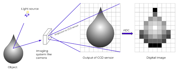
In computer science, the computer sees the images as the nD-array of pixel values. You know videos are the sequence of images stacked together to form a moving picture, and hence computer also sees it as it sees the images.

Pixels are the smallest unit of the digital image. Pixel value represents the color value. It ranges from 0 to 255. Through these pixel values, computers/machines try to understand the image provided to them.

One of the major goals of CV is to bridge the gap between the pixels and meaning. It tries to create meaningful information from the nD-array of pixels values.

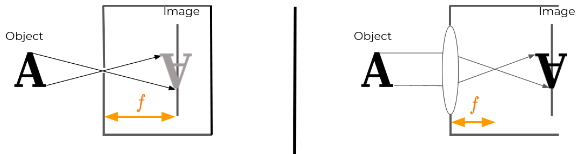
Image formation:

Image of an object is formed when a light reflected from that object is captured by an image capturing devices like human eyes, camera. For the image of an object to be formed, it requires light striking the object and the reflected light being captured by an eye or an camera.

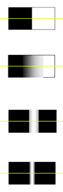
A pixel is a discrete element of a digital image:

Image Type	Representation	Pixel Value
Binary image	$2 D$ -matrix	Binary ${0, 1}$
Grayscale image	$2 D$ -matrix	Discrete - ${0, 1, 2, \dots, 255}$
Colored image	$3 D$ -tensor	R- ${0, 1, \dots 255}$ ; G- ${0, 1, \dots 255}$ ; B- ${0, 1, \dots 255}$

CIELab Color Space:

Unlike other color spaces like RGB, CMY, etc. which were designed to meet device requirements for producing colors (e.g., how much colorants to use to produce an image in a printer or monitor screen). CIELab was based on human vision and not on any particular device. Hence, it’s device independent.

it’s calorimetric, meaning colors that are perceived as matching are encoded identically.

CIELab has three components:

L* - indicates the luminosity of the colors. Its range from 0 to 100, usually with 0 indicating very low intensity and 100 indicating high intensity.
a* - represents the green-red axis, its values range from -127 to +127 such that colors near -127 are green and near +127 are red.
b* - it represents the blue-yellow axis., its values range from -127 to +127, with -127 representing blue and +127 representing yellow colors.

In OpenCV, all the components are scaled to range 0 to 255.

Projections:

(see computer graphics notes)

Rotation, Scaling, Translation: (notice where basis vectors land)

For this, OpenCV provide functions cv.getRotationMatrix2D and cv.warpAffine to apply the affine transformation. Affine transformation include the transformation like scaling, rotation, translation, shearing, reflections, where linear mapping is done such that it preserves the lines and parallelism.

Image Processing

is a method of performing certain image operations to obtain an enhanced image or extract some useful information from it.

Point operators (pixel transforms)
Neighborhood (area-based) operators/filters

Point operators: includes

Brightness and contrast adjustment
Color correction and color transformation

`color_img = cv2.convertScaleAbs(img, alpha = 2.5, beta = 10)

plt.hist(img.flatten(), max_val, [min_val,max_val])

Mask:

`cv2.rectangle(img, pt1=(210,30), pt2=(570,410), color=(255,0,0), thickness=8)

Thresholding: is a type of image segmentation in which you segment the image into the foreground and background.

Binary thresholding: creates a binary image where a value below the threshold is 0, and above threshold is 255. _, THRES_BINARY = cv2.threshold(bimodal_image, global_thres, max_val, cv2.THRESH_BINARY)

where, global_thres set manually from image histogram;

Otsu thresholding: where a threshold value for a bimodal image is calculated automatically from the image histogram.

Local adaptive thresholding: a global threshold will not work when different images have different lightning conditions and exposures.

Resizing

nearest neighbor
bi-linear
bi-cubic

cv2.resize(img, dimension, interpolation = cv2.INTER_AREA)

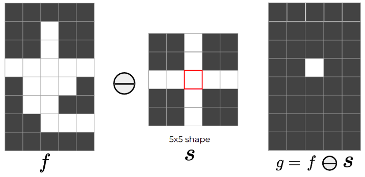
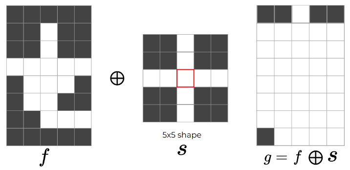
Morphological Processing

Mathematical concept of set-theory: one is the image object, and the other is a structuring element

(primarily for binary images, applicable to color images too - not sure how)

Erosion:

erodes the boundary, shrinks the areas of foreground pixels;
eliminates narrow regions,
thinns the wider ones;

Properties:

Translation equivariant

Dilation:

opposite (not inverse) of erosion

Properties:

Translation equivariant

Convolution

measures the effect of a kernel on the input signal;

dst = cv2.filter2D(img, -1, kernel) kernel =

Blurring:

Box filter (moving average): np.ones((5,5),np.float32)/25
Gaussian sampling: gk = cv2.getGaussianKernel(ksize=3, sigma=10); np.dot(gk, gk.T)

Deblurring/sharpening:

(add detected edge to original image)

Edge Detection

Edge types:

Sobel:

Different gradient operators estimate image gradients from the input image or a smoothed version of it. $L_{x} (x, y) = - \frac{1}{2} L (x - 1, y) + 0 \cdot L (x, y) + \frac{1}{2} L (x + 1, y)$ $L_{y} (x, y) = - \frac{1}{2} L (x, y - 1) + 0 \cdot L (x, y) + \frac{1}{2} L (x, y + 1)$

Classical detectors:

np.array([[-1, -1, -1], [-1, 8, -1], [-1, -1, -1]]);

Canny edge detectors:

Not sensitive to noise.
Combines derivative and smoothing properties in a suitable way.
Adjustable parameters: Width of Gaussian, Low threshold, High threshold

Steps:

Apply Gaussian filter to smooth the image in order to remove the noise.
Find the intensity gradients of the image.
Apply gradient magnitude thresholding or lower bound cut-off suppression to get rid of spurious response to edge detection.
Apply double threshold to determine potential edges.
Track edges by hysteresis: Finalize the detection of edges by suppressing all the other edges that are weak and not connected to strong edges.

canny = cv2.Canny(img, 100, 200) #threshold1,2

Feature Detection

Global features:

multi-dimensional feature vector which describes the overall information in the image
can not distinguish foreground from the background of an image
fail to describe mixture of information from different parts of an image
not robust to occlusions, changes in brightness or viewpoint, image distortions, etc.

Local features:

Localized features or points that stand out.
Invariant to image transformations like rotation, shrinking, expanding, translation, distortion etc.

Harris:

Corners are considered as one of the distinctive and appropriate features:

Corners are regions in the image with large variations in intensity in all the directions. (some way…)

The Harris corner is not rotation invariant. SIFT fixes that.

SIFT:

(even weird way…)

(not even opencv supports it…)

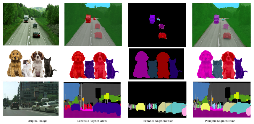
Segmentation

Segmentation creates a pixel-wise mask for each objects in the image.

Types:

Semantic: assigns a same pixel values to a corresponding classes
Instance:
Panoptic:

(split and merge …)

(K-Means)

(to be continued …) Others:

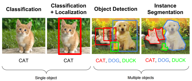
Classification

Localization

Detection

…

Object localization and detection

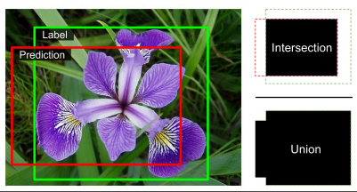
Object localization involves the process of identifying a specific object category within an image, usually by defining a closely cropped bounding box that encompasses the object. One common method to achieve this is by forecasting the object’s center coordinates along both the horizontal and vertical axes, as well as its height and width, in order to predict the bounding box that surrounds the object.

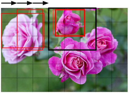
The task of classifying and localizing multiple objects in an image is called object detection. A common approach was to take a CNN that was trained to classify and locate a single object, then slide it across the image. Some post-processing will then be needed to get rid of all the unnecessary bounding boxes.

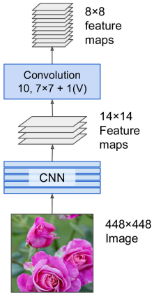
The only difference between FC and CONV layers is that neurons in the CONV layer are connected only to a local region in the input, and that many of the neurons in a CONV volume share parameters. The ability to convert an FC layer to a CONV layer is particularly useful in practice.

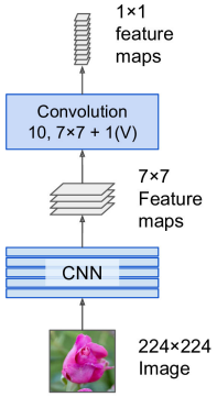
Consider a ConvNet architecture that takes a $224 \times 224 \times 3$ image, and then uses a series of CONV layers and POOL layers to reduce the image to an activation volume of size $7 \times 7 \times 512$ . From there, uses two FC layers of size $4096$ and finally the last FC layers with $1000$ neurons that compute the class scores.
Replace the first FC layer that looks at $[7 \times 7 \times 512]$ volume with a CONV layer that uses filter size $F = 7$ giving output volume $[1 \times 1 \times 4096]$
Replace the second FC layer with a CONV layer that uses filter size $F = 1$ , giving output volume $[1 \times 1 \times 4096]$
Replace the last FC layer similarly, with $F = 1$ , giving final output $[1 \times 1 \times 1000]$ .
Note that instead of a single vector of class scores of size $[1 \times 1 \times 1000]$ , we’re now getting an entire $6 \times 6$ array of class scores across the $384 \times 384$ image.
If we now feed a $448 \times 448$ image, the FCN will process the whole image only once and it will output $8 \times 8$ grid. It’s exactly like taking the original CNN and sliding it across the image using $8$ steps per row and $8$ steps per column: to visualize this image, chopping the original image into a $14 \times 14$ grid, then sliding a $7 \times 7$ window across the grid: there will be $8 \times 8$ predictions.

Semantic segmentation

Semantic Segmentation is a task in which the goal is to categorize each pixel in an image into a class or object. This produces a dense pixel-wise segmentation map of an image, where each pixel is assigned to a specific class or object.

A simple solution proposes to start by taking a pretrained CNN and turning into an FCN. The CNN applies a stride of 32 to the input image overall (i.e., if you add up all the strides greater than 1), meaning the last layer outputs feature maps that are 32 times smaller than the input image.

This is clearly too coarse, so they add a single upsampling layer that multiplies the resolution by $32$ .

There are several solutions available for upsampling (increasing the size of an image), such as:

Bilinear interpolation:

Transposed convolutional layer: equivalent to first stretching the image by inserting empty rows and columns full of zeros, then performing a regular convolution. The transposed convolutional layer can be initialized to perform to linear interpolation, but since it is a trainable layer, it will learn to do better during training.

UNet?

…

Vision Transformers

(2020 oct, after GPT 3)

idea: lets not do local attention over pixels but do global attention over patches each of size 16 by 16, the paper shows advantages are that transformer can attain to far away pixels in the beginning only while CNN would normally take some far away

A pure transformer applied directly to sequences of image patches can perform very well on image classification tasks. When pre-trained on large amounts of data and transferred to multiple mid-sized or small image recognition bechmarks (ImageNet, CIFAR-100, VTAB, etc.), ViT attains excellent results compared to state-of-the-art convolutional neural networks while requiring substantially fewer computational resources to train.

Inspired by Transformer scaling successes in NLP, we experiment applying a standard Transformer directly to images, with the fewest possible modifications. To do so, we split an image into patches and provide the sequence of linear embeddings of these patches as an input to a Transformer. Image patches are treated the same way as tokens in an NLP application. We train the model on image classification in supervised fashion.

When trained on mid-sized datasets such as ImageNet (1M samples 10k classes) without strong regularization, these models yield modest accuracies of a few percentage points below ResNets of comparable size. This seemingly discouraging outcome may be expected: Transformers lack some of the inductive biases inherent to CNNs, such as translation equivariance and locality, and therefore do not generalize well when trained on insufficient amount of data.

However, the picture changes if the models are trained on larger datasets (14M-300M). We find that large scalar training trumps inductive bias. Our ViT attains excellent results when pre-trained at sufficient scale and transferred to tasks with fewer datapoints. When pre-trained on public ImageNet-21k dataset or in house JFT-300M dataset, ViT approaches or beats state of art on multiple image recognition benchmarks.

Lastly, we perform a small experiment using self-supervision, and show that self-supervised ViT holds promise for the future.

Naive application of self-attention to images would require that each pixel attends to every other pixel. With quadratic cost in the number of pixels, this does not scale to realistic input sizes.

(something about combining CNN and stuffs)

The standard transformer receives as input a 1D sequence of token embeddings. To handle 2D images, we reshape the image $x \in R^{H \times W \times C}$ into a sequence of flattened 2D patches, $x_{p} \in R^{N \times (P^{2} C)}$ , where (H, W) is the resolution of the original image, C is the number of channels, (P, P) is the resolution of each image patch, and $N = H W / P^{2}$ is the resulting number of patches, which also serves as the effective input sequence length for the transformer. The Transformer uses constant latent vector size D through all of its layers, so we flatten the patches and map to D dimensions with a trainable linear projection: $z_{0} = [x_{class}; x_{p}^{1} E; x_{p}^{2} E; \dots; x_{p}^{N} E] + E_{pos}$ The resulting sequence of embedding vectors serve as input to the encoder. (Now from the transformer comes out these equations: pre norm and GLEU non-linearity) $z_l'=MSA(LN(z_{l-1}))+z_{l-1},~l=1,\ldots,L$$$$z_l=MLP(LN(z'_l)+z'_l),~l=1,\ldots,L$ $y = L N (z_{L}^{0})$ We note that ViT has much less image-specific inductive bias than CNNs. In CNNs, locality, two-dimensional neighborhood structure, and translational equivariance are baked into each layer throughout the whole model. In ViT, only MLP layers are local and translationally equivariant, while the self-attention layers are global. The two-dimensional neighborhood structure is used very sparingly; in the beginning of the model by cutting the image into patches and at fine-tuning time for adjusting the position embeddings for images of different resolution. Other than that, the position embeddings at initialization carry no information about the 2D positions of the patches and all spatial relations between the patches have to be learned from scratch.

(so this is supervised pretraining right?)

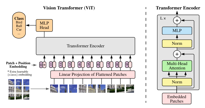
Typically, we pre-train ViT on large datasets, and fine-tune to (smaller) downstream tasks. For this, we remove the pre-trained prediction head and attach a zero-initialized D × K feedforward layer, where K is the number of downstream classes. It is often beneficial to fine-tune at higher resolution than pre-training. When feeding images of higher resolution, we keep the patch size the same, which results in a larger effective sequence length. The Vision Transformer can handle arbitrary sequence lengths (up to memory constraints), however, the pre-trained position embeddings may no longer be meaningful. We therefore perform 2D interpolation of the pre-trained position embeddings, according to their location in the original image. Note that this resolution adjustment and patch extraction are the only points at which an inductive bias about the 2D structure of the images is manually injected into the Vision Transformer.

(something called big transfer is there) Datasets:

To explore model scalability, we use the ILSVRC-2012 ImageNet dataset with 1k classes and 1.3M images, its superset Imagenet-21k with 21k classes and 14M images, and JFT with 18k classes and 303M high-resolution images.
We de-duplicate the pre-training datasets w.r.t the test sets of the downstream tasks.
We transfer the models trained on these datasets to several bechmark tasks (some shits)

Swin transformer

(2021 march)

This paper presents a new vision Transformer, called Swin Transformer, that capably serves as a general purpose backbone for computer vision. Challenges in adapting Transformer from language to vision arise from differences between the two domains, such as:

Large variations in the scale of visual entities. Unlike the word tokens that serve as the basic elements of processing in language transformers, visual elements can vary substantially in scale. In existing transformer-based models, tokens are all of a fixed scale, a property unsuitable for these vision applications.
High resolution pixels in images compared to words in text. There exists many vision tasks such as semantic segmentation that require dense prediction such as semantic segmentation that require dense prediction at pixel level, and this would be intractable for transformer on high-resolution images, as the computational complexity of its self-attention is quadratic to image size.

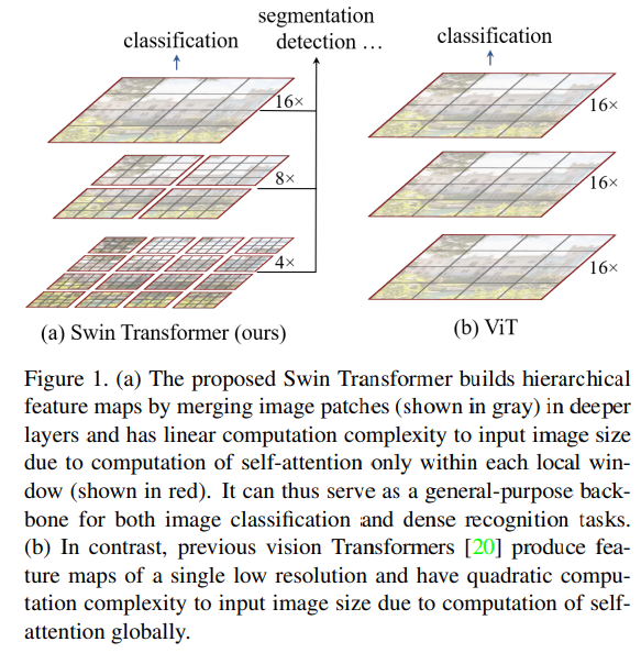
To address these differences, we propose a Transformer backbone, called Swin Transformer, which constructs hierarchical feature maps and has linear computational complexity to image size.

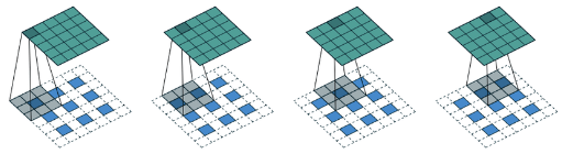
The Swin constructs a hierarchical representation by starting from small-size patches (gray boundaries) and gradually merging neighboring patches in deeper Transformer layers. With these hierarchical feature maps, the Swin Transformer model can conveniently leverage advanced techniques for dense prediction such as feature pyramid networks (FPN or U-Net). The linear computational complexity is achieved by computing self-attention locally with non-overlapping windows that partition an image (outlined in red).

A key design element of Swin Transformer is its shift of the window partition between consecutive self-attention layers. The shifted windows bridge the windows of the preceding layer, providing connections among them that significantly enhance modeling power. This strategy is also efficient in regards to real-world latency: all query patches within a window share the same key set, which faciliates memory access in hardware. In contrast, earlier sliding window based self-attention approaches, suffer from low latency on general hardware due to different key sets for different query pixels.

(about results and related works)

Architecture:

It first applies an input RGB image into non-overlapping patches by a patch splitting module, like ViT. Each path is treated as a token and its feature is set as a concatenation of the raw RGB pixel values. In our implementation, we use a patch size of 4 × 4 and thus the feature dimension of each patch is 4 × 4 × 3 = 48. A linear embedding layer is applied on this raw-valued feature to project it to an arbitrary dimension (denoted as C).

Several Transformer blocks with modified self-attention computation (Swin Transformer blocks) are applied on these patch tokens. The Transformer blocks maintain the number of tokens ( $\frac{H}{4} \times \frac{W}{4})$ , and together with the linear embedding referred to as stage 1.

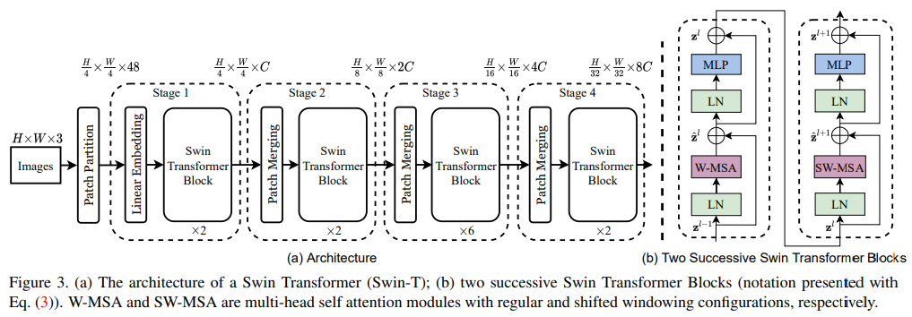
To produce a hierarchical representation, the number of tokens is reduced by patch merging layers as the network gets deeper. The first patch merging layer concatenates the features of each group of $2 \times 2$ neighboring patches, and applies a linear layer on the 4C dimensional concatenated features. This reduces the number of tokens by a multiple of 2x2=4 (2 x downsampling resolution), and the output dimension is set to 2C. Swin Transformer blocks are applied afterwards for feature transformation, with the resolution kept at $\frac{H}{8} \times \frac{W}{8}$ . This first block of patch merging and feature transformation is denoted as “Stage 2”. The procedure is repeated twice as “Stage 3” and “Stage 4”, with output resolutions of $\frac{H}{16} \times \frac{W}{16}$ and $\frac{H}{32} \times \frac{W}{32}$ , respectively. These stages jointly produce a hierarchical representation, with the same feature map resolutions as those of typical convolutional networks.

Whats inside these Swin blocks?

Swin Transformer is built by replacing the standard multi-head self attention (MSA) module in a Transformer by a module based on shfited windows, with other layers kept the same. A Swin Transformer block consits of a shifted window based MSA module, followed by a 2-layer MLP with GLEU non linearity in between. A LayerNorm (LN) layer is applied before each MSA module and each MLP, and a residual connection is applied after each module.

For efficient modeling, we propose to compute self-attention within logical windows. The windows are arranged to evenly partition the image in a non-overlapping manner. Supposing each window contains $M \times M$ patches, the computational complexity of a global MSA module and a window based one on an image of $h \times w$ patches are: $Ω (MS A) = 4 h w C^{2} + 2 (h w)^{2} C$ $Ω (W - MS A) = 4 h w C^{2} + 2 M^{2} h wC$ where the former is quadratic to patch number $h w$ , and the latter is linear when $M$ is fixed (set to 7 by default). Global self-attention computation is generally unaffordable for a large $h w$ , while the window based self-attention is scalable.

The window-based self-attention module lacks connections across windows, which limits its modeling power. To introduce cross-window connections while maintaining the efficient computation of non-overlapping windows, we propose a shifted window portioning approach which alternates between two partitioning configurations in consecutive Swin Transformer blocks.

As shown below, the first module uses a regular window partitioning strategy which starts from the top-left pixel, and the $8 \times 8$ feature map is evenly partitioned into $2 \times 2$ windows of size $4 \times 4 (M = 4)$ . Then, the next module adopts a windowing configuration that is shifted from that of the preceding layer, by displacing the windows by $(⌊ \frac{M}{2} ⌋, ⌊ \frac{M}{2} ⌋)$ pixels from the regularly partitioned windows.

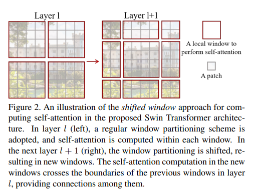(the second window is bigger, imagine it)

With the shifted window partitioning approach, consecutive Swin Transformer blocks are computed as: (some equations)

(stuffs)

Experiments: (some augmentation and other techniques rey)

Regular ImageNet-1K training vs ImageNet-22K pre-training: For Swin-B, the ImageNet22K pre-training brings 1.8%∼1.9% gains over training on ImageNet-1K from scratch. Compared with the previous best results for ImageNet-22K pre-training, our models achieve significantly better speed-accuracy trade-offs: Swin-B obtains 86.4% top-1 accuracy.

(I mean if you remember, the object detection and segmentation are done with CNN networks as backbones, so they do comparison of Swin and Resnet as backbones on these tasks)

CLIP

(feb 2021, before swin) (how about embedding text and image in same space?)

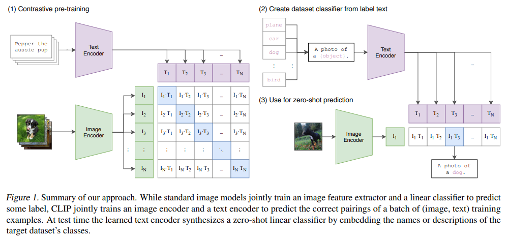
Computer vision systems are trained to predict a fixed set of predetermined object categories. This restricted form of supervision limits their generality and usability since additional label data is needed to specify any other visual concept. Learning directly from raw text about images is a promising alternative which leverages a much broader source of supervision. We demonstrate that the simple pre-training task of predicting which caption goes with which image is an efficient and scalable way to learn SOTA image representations from scratch on a dataset of 400 million (image, text) pairs collected from the internet.

After pre-training, natural language is used to reference learned visual concepts (or describe new ones) enabling zero-shot transfer of the model to downstream tasks. The model transfers non-trivially to most tasks and is often competitive with a fully supervised baseline without the need for any dataset specific training. For instance, we match the accuracy of the original ResNet-50 on ImageNet zero-shot without needing to use any of the 1.28 million training examples it was trained on.

Task agnostic objectives such as autoregressive and masked language modelling have scaled across many orders of magnitude in compute, model capacity, and data, steadily improving capabilities
The development of text to text (i guess GPT and T5 are the ones) as a standardized input-output interface has enabled task-agnostic architecture to zero-shot transfer to downstream datasets removing the need for specialized output heads or data specific customization.

Enabled by the large amounts of publicly available data of this form on the Internet, we create a new dataset of 400 million (image, text) pairs and demonstrate a simplified version trained from scratch, which we call CLIP, for Contrastive Language-Image Pre-training, is an efficient method of learning from natural language supervision.

We find that CLIP, similar to the GPT family, learns to perform a wide set of tasks during pre-training including OCR, geo-localization, action recognition, and many others. We measure this by benchmarking the zero-shot transfer performance of CLIP on over 30 existing datasets and find it can be competitive with prior task-specific supervised models.

Approach:

Existing work has mainly used three datasets, MS-COCO, Visual Genome, and YFCC100M.

While MS-COCO and Visual Genome are high quality crowd-labeled datasets, they ware small by modern standards with approximately 100k training photos each. By comparison, other computer vision systems are trained up to 3.5 billion Instagram photos.
YFCC100M, at 100 million photos, is a possible alternative, but metadata for image is sparse and of varying quality. Many images use automatically generated filenames like 12122434.JPG as titles or contain descriptions of camera exposure settings. After filtering, the dataset shrunk by 6 to only 15 million photos.

To address this, we constructed a new dataset of 400 million (image, text) pairs collected from a variety of publicly available sources on the Internet. To attempt to cover as broad a set of visual concepts as possible, we search for (image, text) pairs as part of the construction process whose text includes one of a set of 500,000 queries. The base query list is all words occurring at least 100 times in the English version of Wikipedia. We approximately class balance the results by including up to 20,000 (image, text) pairs per query. The resulting dataset has a similar total word count as the WebText dataset used to train GPT-2. We refer to this dataset as WIT for WebImageText. (i dont think its public yet)

Pre-training method:

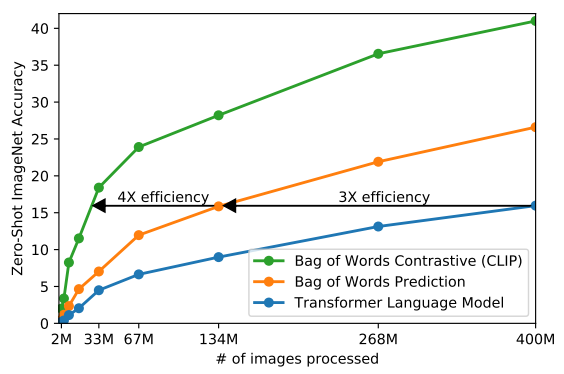
In the course of our efforts, we found training efficiency was key to successfully scaling natural language supervision and we selected our final pre-training method on this metric.

Our initial approach jointly trained an image CNN and text transformer from scratch to predict caption of an image. However, we encountered difficulties efficiently scaling this method. A 64M parameter transformer language model, which already uses twice the compute of its ResNet-50 image encoder, learns to recognize ImageNet classes three times slower than a much simpler baseline that predicts a bag-of-words encoding of the same text.
They try to predict the exact words of the text accompanying each image. This is a difficult task due to the wide variety of descriptions, comments, and related text that co-occur with images.
Recent work in contrastive representation learning for images has found contrastive objectives can learn better representations than their equivalent predictive objective. Other work has found that although generative models of images can learn high quality image representations, they require over an order of magnitude more compute thatn contrastive models with the same performance.
Noting these findings, we explored training a system to solve the potentially easier proxy task of predicting only which text as a whole is paired with which image and not the exact words of that text.

(so basically constrative vs predictive vs generative; they learn representations)

Given a batch of $N$ (image, text) pairs, CLIP is trained to predict which of the $N \times N$ possible (image, text) pairings across a batch actually occurred. To do this, CLIP learns a multi-modal embedding space by jointly training an image encoder and text encoder to maximize the cosine similarity of the image and text embeddings of the $N$ real pairs in the batch while minimizing the cosine similarity of the embeddings of the $N^{2} - N$ incorrect pairings. We optimize a symmetric cross entropy loss over these similarity scores.

(pseudo code is here, that shows that you can have pretrained image and text encoder)

We train CLIP from scratch without initializing the image encoder with ImageNext weights or the text encoder with pre-trained weights. We use only a linear projection to map from each encoder’s representation to the multi-modal embedding space. (some things about how it is different from similar works)

(some details, like text was transformer while image was tested with resnet and vit)

Zero-shot transfer: While GPT-1 focused on pretraining as a transfer learning method to improve supervised fine-tuning, it also included an ablation study demonstration that the performance of four heuristic zero-shot transfer methods improved steadily over the course of pre-training, without any supervised adaptation. This analysis served as the basis of GPT-2 which focused exclusively on studying the task-learning capabilities of language models via zero-shot transfer.

CLIP is pre-trained to predict if an image and a text snipped are paired together in its dataset. To perform zero-shot classification, we reuse this capability. For each dataset, we use the names of all the classes in the dataset as the set of potential text pairings and predict the most probable (image, text) pair according to CLIP. In a bit more detail, we first compute the feature embedding of the image and the feature embedding of the set of possible texts by their respective encoders. The cosine similarity of these embeddings is then calculated, scaled by a temperature parameter τ , and normalized into a probability distribution via a softmax. (whatever whatever I get the idea now)

(about results)

Prompt engineering:

A common issue is polysemy. When the name of a class is the only information provided to CLIP’s text encoder it is unable to differentiate which word sense is meant due to the lack of context. In some cases multiple meanings of the same word might be included as different classes in the same dataset! This happens in ImageNet which contains both construction cranes and cranes that fly. Another example is found in classes of the Oxford-IIIT Pet dataset where the word boxer is, from context, clearly referring to a breed of dog, but to a text encoder lacking context could just as likely refer to a type of athlete.

Another issue we encountered is that it’s relatively rare in our pre-training dataset for the text paired with the image to be just a single word. Usually the text is a full sentence describing the image in some way. To help bridge this distribution gap, we found that using the prompt template “A photo of a {label}.” to be a good default that helps specify the text is about the content of the image. This often improves performance over the baseline of using only the label text. For instance, just using this prompt improves accuracy on ImageNet by 1.3%.

Similar to prompt engineering discussion aroung GPT-3, we have also observed that zero-shot performance can be significantly improved by customizing the prompt text to each task. A few, non exhaustive, examples follow. We found on several fine-grained image classification datasets it helped to specify the category.

For example on Oxford-IIIT pets, using “A photo of a {label}, a type of pet.” to help provide context worked well.
Likewise, on Food101 specifying a “type of food” and on FGVC Aircraft “a type of aircraft” helped too.
For OCR datasets, we found hat putting quotes around the text or number to be recognized improved performance.
Finally, we found that on satellite image classification datasets it helped to specify that the images were of this form and we use variants of “a satellite photo of a {label}.”.

(aru yestai yestai guff haru pani xan hai)

From youtube video:

Well, we could do this other way as well, that given an text and images. Tell which image is closer.
This requires large minibatch right?
People guide GAN using this rey
This performs poorly on MNIST lmao, there is graph
Zero shot clip has some performance, and it decreases as you do linear proabing firs then only starts to increase as we move to couple of examples, because there is some intuitive explanation
Some performance are bad on certain datasets when there are no images in internet
Info about how performance of models as we scale compute/data
Robustness to shift: There are variations of ImageNet:

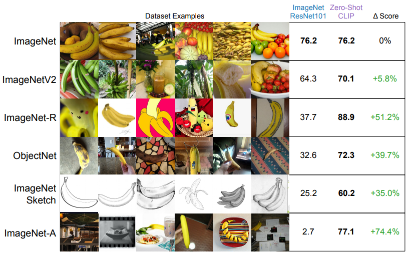
Other models trained on ImageNet, perform really poorly on this adversial type of images. But CLIP is doing pretty well. The data shows. So, it is quite robust.
The reason is simple. The specifically trained network remembers only the dataset it was trained on, if you show it picture of banana. It gets mad because it knows banana are only yellow.
You can also linear probe CLIP on ImageNet by only midly degrading performance on other datasets
Also, there is a limitation section on how you engineer the prompt

FLaVa

(Like CLIP)

BiomedCLIP

(CLIP specifically made from scratch using medical images)

CLIPSeg

(2021 Dec)

Abstract:

Image segmentation is usually addressed by training a model for a fixed set of object classes. Incorporating additional classes or more complex queries later is expensive as it requires re-training the model on a dataset that encompasses these expressions. Here we propose a system that can generate image segmentation based on arbitrary prompts at test time.

A prompt can be either a text or an image. This approach enables us to create a unified model (trained once) for three common segmentation tasks, which come with distinct challenges:

referring expression segmentation,
zero-shot segmentation, and
one-shot segmentation.

We build upon the CLIP model as a backbone which we extend with a transformer-based decoder that enables dense prediction. After training on an extended version of the PhraseCut dataset, our system generates a binary segmentation map for an image based on a free-text prompt or on an additional image expressing the query.

Details:

Image segmentation requires a model to output a prediction for each pixel. Compared to whole-image classification, segmentation requires not only predicting what can be seen but also where it can be found. Classification semantic segmentation models are limited to segment the categories they have been trained on.

In generalized zero-shot segmentation, seen as well as unseen categories needs to be segmented by putting unseen categories in relation to seen ones.
In one-shot segmentation, the desired class is provided in form of an image (and often an associated mask) in addition to the query image to be segmented
In referring expression segmentation, a model is trained on complex text queries but sees all classes during training (i.e. no generalization to unseen classes)

We introduce the CLIPSeg model which is capable of segmenting based on an arbitrary text query or an example image. CLIPSeg can address all three tasks named above. To realize this system, we employ the pre-trained CLIP model as a backbone and train a thin conditional segmentation layer (decoder) on top. We use the joint textvisual embedding space of CLIP for conditioning our model, which enables us to process prompts in text form as well as images. Our idea is to teach the decoder to relate activations inside CLIP with an output segmentation, while permitting as little dataset bias as possible and maintaining the excellent and broad predictive capabilities of CLIP.

We employ a generic binary prediction setting, where a foreground that matches the prompt has to be differentiated from background.

Related work: (foundational models, generic, zero-shot, one-shot)

ClipSeg:

We use the visual transformer-based CLIP model as a backbone and extend it with a small, parameter-efficient transformer decoder. The decoder is trained on custom datasets to carry out segmentation, while the CLIP encoder remains frozen. A key challenge is to avoid imposing strong biases on predictions during segmentation training and maintaining the versatility of CLIP. (larger ones weights are not released)

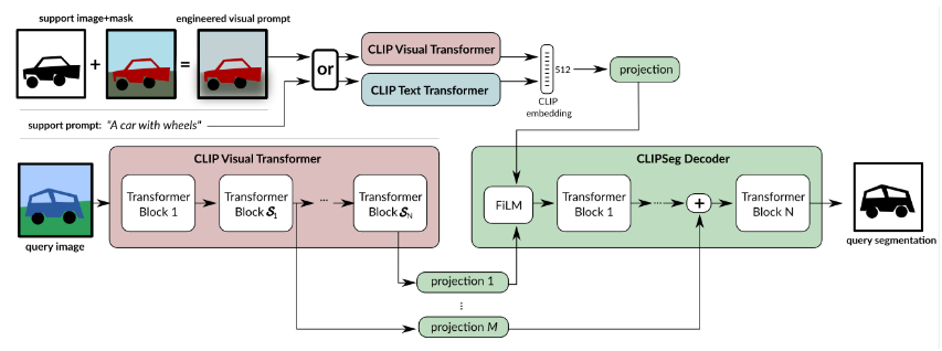
Considering these demands, we propose CLIPSeg: A simple, purely-transformer based decoder, which has U-Net inspired skip connections to the CLIP encoder that allow the decoder to be compact (in terms of parameters).

While the query image ( $R^{W \times H \times 3})$ is passed through the CLIP visual transformer, activation at certain layers $S$ are read out and projected to the token embedding size $D$ of our decoder. Then, these extracted activations (including CLS token) are added to the internal activations of our decoder before each transformer block. The decoder has as many transformer blocks as extracted CLIP activations (in our case 3). The decoder generates the binary segmentation by applying a linear projection on the tokens of its transformer (last layer) $R^{(1 + \frac{W}{P} \times \frac{H}{P}) \times D)} \to R^{W \times H}$ , where $P$ is the token patch size of CLIP.

In order to inform the decoder about the segmentation target, we modulate the decoder’s input activation by a conditional vector using FiLM. This conditional vector can be obtained in two ways:

Using the CLIP text-transformer embedding of a text query and
Using the CLIP visual transformer on a feature engineered prompt image CLIP itself is not trained, but only used as a frozen feature extractor. Due to the compact decoder, CLIPSeg has only 1,122,305 trainable parameters for D=64.

The original CLIP is constrained to a fixed image size due to the learned positional embedding. We enable different image sizes (including larger ones) by interpolating the positional embeddings

Image-Text Interpolation: Our model receives information about the segmentation target (what to segment?) through a conditional vector. This can be provided either by text or an image (through visual prompt engineering). Since CLIP uses a shared embedding space for images and text captions, we can interpolate between both in the embedding space and condition on the interpolated vector.

…

Under the hood, CLIPSeg leverages OpenAI’s powerful CLIP image-text model that enables seamless use of text-prompting for computer vision tasks. CLIP equips CLIPSeg with the following image segmentation tasks:

Referring segmentation: Segment an image based on text prompts that the model has seen during training.
Zero-shot segmentation: Segment an image based on novel open-vocabulary prompts that has not seen during training.
One-shot segmentation: Segment an image by showing it a prototype image of an object of interest.

Its text and visual prompting capabilities enable CLIPseg to work as an agent with large language models like GPT-4 to facilitate many business use cases.

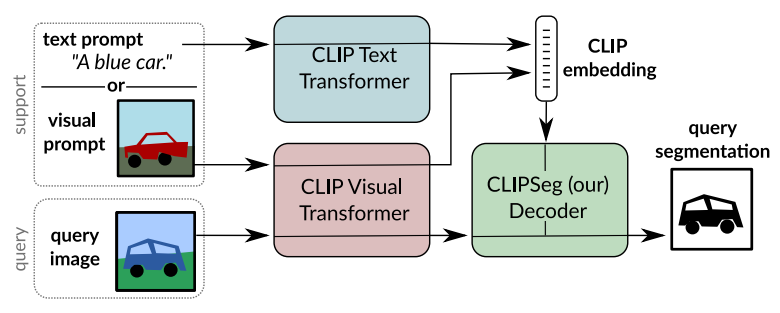
(along top line, you can see that either you send “a car with wheels” or just image of it, since they are on same embedding space, it works)

CLIPSeg has a transformer-based, encoder-decoder architecture. Its encoder is a pre-trained CLIP vision-language model based on the vision transformer (ViT-B/16) network. It generates an embedding and attention activations for a target image.

For the decoder, CLIPSeg stacks three standard transformer blocks that combine the target image embedding, its activations, and the conditioning prompt to output a binary segmentation mask.

Encoder-decoder connections:

A single embedding, generated by the encoder for a target image, is insufficient to identify precise segmentation masks. A lot of useful information required by the decoder is not available in the embedding. However, it is available in the attention activations of the encoder’s transformers blocks.

So CLIPSeg opts for a U-Net-like architecture where its three decoder blocks are connected to three of the vision transformer encoder’s blocks. Their attention information enables the decoder blocks to more accurately infer both nearby and distant spatial and semantic relationships in the image.

Conditioning on prompts with feature-wise linear modulation:

Text and image prompts are additional multi-modal inputs that the model must combine with a target image in some way. Influencing a model’s results in this fashion, with additional input, is called ‘conditioning’. For example. a popular conditioning technique for natural language processing (NLP) combines token position embeddings with input text embeddings. But that approach just influences the first layer.

Conditioning techniques that influence not just the first but every layer of the model give better results. CLIPSeg uses one such technique called feature-wise linear modulation (FiLM).

FiLM works as follows:

It obtains the feature maps from a selected transformer block in the CLIP encoder. We will call this feature matrix $F (i, c)$ , indicating that its the $c$ th feature map for the $i$ th input token. Since we are talking about visual transformers here, the $i$ th input token is just the $i$ th image patch.
It applies an affine transformation $γ (i, c) \cdot F (i, c) + β (i, c)$ - to the layer’s feature map to generate a new conditioned feature map.
(I guess yeha ta c huni kura bhayena because we consider entire 768 as c, just $γ (i) \cdot F (i) + β (i)$ huni bhayo)
$γ$ and $β$ are feature-wise weights produced by two arbitrary functions applied on the conditioning prompt. They are different for each feature map - hence the term feature-wise.
In practice $γ$ and $β$ are learned by two linear layers of the CLIPSeg model during training. During inference, these layers generate the conditioning weights from a given prompt.
Since they’re obtained using an affine transform, the new feature maps will retain the spatial relationships of the original feature maps.

(some other shits) How zero shot and few shot segmentation with text prompts and visual prompts works:

Zero-shot text-guided segmentation is when the text prompt you supply is not part of the CLIP dataset or training. It’s a novel prompt that CLIPSeg is seeing for the first time. Despite that, it infers visual concepts that are semantically related to that prompt, identifies them in the query image, and segments them with the following steps:

Get a CLIP embedding for the text or text and image prompt:

In zero-shot environments the supplied text prompt is run through CLIP’s text encoder to obtain an embedding vector. This is a bit different in few-shot as a visual prompt consisting of the example object and its mask is run through CLIP’s visual encoder. Note that this is not a simple image processing operation of isolating the object using the object mask and then obtaining an embedding for the isolated object. Instead, the object mask must condition the multi-head attention weights themselves so that attention is restricted to the image patches in the unmasked areas while ignoring the masked areas.

Run the target image through the CLIP encoder blocks

The target image to segment is run through CLIP’s visual encoder network, which is just a vision transformer ViT-B/32 model by default. However, its goal is not to obtain an embedding for the image.

Extract attention activations from selected encoder blocks

Instead, it’s interested in the attention activations of the third, sixth and ninth encoder blocks to act as sources of skip connections to the decoder blocks. To keep the decoder model light, just these three blocks are selected, but more can be added for improved accuracy.

Condition the activations with the prompt using film

Next, CLIPSeg conditions the last selected encoder block’s activations on the prompt embedding (from the first step) using FiLM. The prompt embedding is supplied to the two FiLM layers to obtain $γ$ and $β$ matrices. They are combined with the encoder block’s activations through an affine transform.

Pass FiLM’s conditioned results through the decoder stack

By default, the CLIPSeg decoder has three transformer blocks:

First decoder block: Uses the conditioned features from the previous step and combines them with the activations from its skip connection to the ninth encoder block
Second decoder block: Combines the first block’s activations with the activations from its skip connection to the sixth encoder block
Third decoder block: Combines the second block’s activations with the activations from its skip connection to the first encoder block

Generate a Segmentation Mask From the Mask Tokens

The final steps convert these mask tokens to a binary segmentation mask that’s the same size as the target image. It does this using a transposed convolution layer (or a couple of them). These layers, also called deconvolution layers, upsample the decoder’s mask tokens to a binary segmentation mask that’s the same size as the image.

Training: We use the PhraseCut dataset, which encompasses over 340k phrases with corresponding image segmentations.

(for image they do something and calls it PC+)

(more things and others, too complicated looks like, but could be)

CRIS

(30 Nov, 2021); older than clipseg) (diff on utilization of CLIP is that CRIS uses resnet clip while clipseg uses vit)

Referring image segmentation aims to segment a referent via a natural linguistic expression. Due to the distinct data properties between text and image, it is challenging for a network to well align text and pixel-level features. Unlike semantic segmentation and instance segmentation, which requires segmenting the visual entities belonging to pre-determined set of categories, referring image segmentation is not limited to indicating specific categories but finding a particular region according to the input language expression.

The direct usage of CLIP can be sub-optimal for pixel-level prediction tasks, e.g., referring image segmentation, due to the discrepancy between image-level and pixel-level prediction. The former focuses on the global information of an input image, while the latter needs to learn fine-grained visual representations for each spatial activation. In this paper, we explore leveraging the powerful knowledge of the CLIP model for referring image segmentation, in order to enhance the ability of cross-modal matching.

(what?) Firstly, we propose a visual-language decoder that captures long-range dependencies of pixel-level features through the self-attention operation and adaptively propagate fine-structure textual features into pixel-level features through the cross-attention operation.

Secondly, we introduce the text-to-pixel contrastive learning, which can align linguistic features and the corresponding pixel-level features, meanwhile distinguishing irrelevant pixel-level features in the multi-modal embedding space. Based on this scheme, the model can explicitly learn fine-grained visual concepts by interwinding the linguistic and pixel-level visual features.

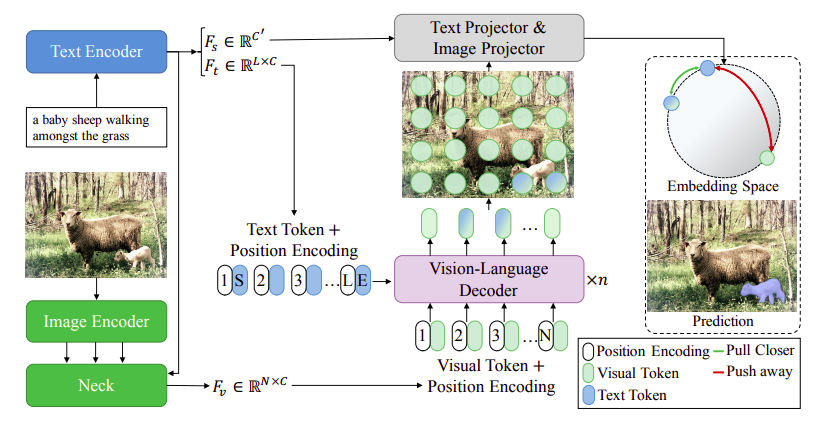
Image and text encoder (from CLIP):

For an input image $I \in R^{H \times W \times 3}$ , we utilize multiple visual features from the 2th-4th stages of the ResNet, which are defined as $F_{v 2} \in R^{\frac{H}{8} \times \frac{W}{8} \times C_{2}}$ , $F_{v 3} \in R^{\frac{H}{16} \times \frac{W}{16} \times C_{3}}$ , and $F_{v 4} = R^{\frac{H}{32} \times \frac{W}{32} \times C_{4}}$ , respectively. Note that $C$ is the feature dimension, $H$ and $W$ are the height and width of the original image.

For an input expression $T \in R^{L}$ , we adopt a Transformer to extract text features $F_{t} \in R^{L \times C}$ . The Transformer operates on a lower cased BPE representation of the text with 49k vocab size, and the text sequence is bracketed with [SOS] and [EOS] tokens. The activations of the highest layer of the transformer at the [EOS] token are further transformed as the global textual representation $F_{s} \in R^{C^{'}}$ . Note that $C$ and $C^{'}$ are the feature dimension, $L$ is the length of the referring expression.

Cross-modal neck:

Given multiple visual features and the global textual representation $F_{s}$ , we obtain the simple multi-modal feature representation $F_{s}$ , we obtain the simple multi-modal features $F_{m 4} \in R^{\frac{H}{16} \times \frac{W}{16} \times C}$ by fusing $F_{v 4}$ with $F_{s}$ : $F_{m 4} = U p (σ (F_{v 4} W_{v 4}) \cdot σ (F_{s} W_{s}))$ where Up(.) denotes $2 \times$ upsampling, $.$ demotes the element-wise multiplication, $σ$ denotes ReLU, $W_{v 4}$ and $W_{s}$ are two learnable matrices to transform the visual and textual representation into the same feature dimension. Then, the multi-modal features $F_{m 2}$ and $F_{m 3}$ are obtained by: $F_{m 3} = [σ (F_{m 4} W_{m 4}), σ (F_{v 3} W_{v 3})]$ (some weird shit I dont get)

Vision-language decoder:

(basically the word embedding from text encoder as cross attention key, while visual from neck as regular input)

We design a vision-language decoder to adaptively propagate fine-grained semantic information from textual features to visual features.

… Fv is first sent into the multi-head self-attention layer to capture global contextual information .. after that, multi-head cross-attention is adopted to propagate fine-grained semantic information into the evolved visual features, … The evolved modal features $F_{c}$ is utilized for the final segmentation mask.

Text-to-pixel contrastive learning:

Although CLIP learns powerful image-level visual concepts by aligning the textual representation with image-level representation, this type of knowledge is sub-optimal for referring image segmentation, due to lack of more fine-grained visual concepts.

To tackle this issue, we design a text-to-pixel contrastive loss, which explicitly aligns the textual features with corresponding pixel-level visual features. $z_{v} = F_{c}^{'} W_{v} + b_{v}, F_{c}^{'} = U p (F_{c})$ $z_{t} = F_{s} W_{t} + b_{t}$ … Given a transformed textual features $z_{t}$ and a set of transformed pixel-level features $z_{v}$ , a contrastive loss is adopted to optimize the relationship between two modalities, where $z_{t}$ is encouraged to be similar with its corresponding $z_{v}$ and dissimilar with other irrelevant $z_{v}$ . With the similarity measured by dot product, the text-to-pixel contrastive loss can be formulated as: …

NAAMII Exploration

Medical image segmentation with deep learning is an important and widely studied topic because segmenation enables quantifying target structure size and shape that can help in disease diagnosis, prognosis, surgery planning, and understanding.

… Compared to visual prompts such as points or boxes, language prompts during inference are, by design, mmore interpretable or explainable and can provide complex auxiliary information regarding texture, shape, and spatial relationships of normal and abnormal structures.

Foundation VLSMs trained on large-scale image-text pairs and the ability to inject auxiliary prompts via language prompt could enable powerful medical image segmentation models that can leverage the separately curated medical datasets (often of small or medium size) by pooled dataset training, adapt to new classes without changing the architecture, provide more explainable results, and potentially have robust human-in-the-loop segmentation systems for out-of-distribution data and domain adaptation.

Quin et al. studied transfer learning for one CLM designed for object detection task, showing promising zero-shot results and surpassing baseline supervised model when finetuning the VLMs with suitable language prompts on small-sized medical images. However, the two critical questions remain unanswered:

How well this holds for the segmentation tasks across multiple VLSMs is unclear. Segmentation is a more difficult task than object detection and arguably more important and ubiquitous in medical imaging because accurate segmentation can provide quantitative measures of target structures.
There is a lack of understanding of the nuanced role of the language prompt vs. image during finetuning and the ability of the VLSMs to handle pooled dataset training and out-of-distribution data.

Image segmentation using foundation vision language models:

Foundation VLMs for medical imaging applications in the literature primarily build upon the VLMs developed with natural images using one of the two approaches:

finetune a pretrained VLM with medical image-text pairs (PubMedCLIP)
pretrain the VLM of the same architecture from scratch with image-tex pairs (MedCLIP, BIomedCLIP)

Although these foundation models are intended to be helpful for a wide range of downstream tasks, their general approach to learning an embedding that aligns the whole image to the entire input text with global embedding is sub-optimal for dense prediction tasks like segmentation.

Segmentation tasks may benefit more from explicitly aligning images and text descriptions. Recent state-of-the-art VLSMs extend CLIP to segmentation tasks by adding a decoder trained to produce a segmentation map from CLIP’s vision and language embeddings. DenseCLIP (need to look into this) has proposed vision language decoders on top of the CLIP encoders that use the pixel-text score maps of the limited class prompts. In contrast to DenseCLIP, CLIPSeg and CRIS enforce zero-shot segmentation by giving the output as pixel-level activations for the given text or image prompt. ZegCLIP (need to look here also) has introduced tune prompts and associated the image information to the text encodings before patch-text contrasting to reduce the seen classes’ overfit

Although there are some specific architectures to learn joint embeddings from image and text prompts for particular datasets, such as TGANet for polyps in endoscopy images, to our knowledge, there are no VLSms well studied for medical images.

Method:

We develop four medical VLSMs using two different strategies:

Finetune two state of the art CLIP-based VLSMs, CLIPSeg and CRIS, that are pretrained on natural image-text pairs.
Building two new VLSMs specific to medical domain by adding a decoder to the foundation CLM BiomedCLIP, pretrained on medical image-text pairs. The two new VLSMs are BiomedCLIPSeg-D - obtained by adding pretrained CLIPSeg decoder to BiomedCLIP (bhanesi same architecture as CLIPSeg right?) and BiomedCLIPSeg obtained by randomly initializing the decoder.

(Two literature architectures, two where they combine CLIPSeg and BiomedCLIP)

These four models are trained on the triplet of medical images, segmentation masks, and text prompts

Real deal

The basic architecture of CRIS and CLIPSeg/BiomedCLIPSeg VLSMs:

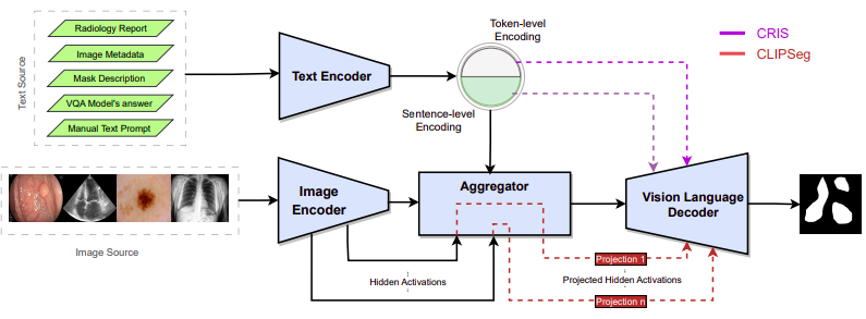
The VLSM consists of a Text Encoder, an Image Encoder, a Vision Language Decoder (VLD), and an Aggregator. The inpu tto the model is a pair of an image and a language prompt fed tot he Image Encoder and Text Encoder respectively. The Aggregator generates intermediate representations utilizing image-level, sentence-level, or word-level representation to feed to the VLD.

CLIPSeg and CRIS were trained on PhraseCut with 340k text-image pairs and RefCOCO with 142,210 text-image pairs, respectively. Architecture-wise, CLIPSeg has the text embedding at the neck of the vision encoder-decoder network.

30210448

My Knowledge Base

Explorer